sagemath.sagews

Sagemath

• symbolic variables

• symbolic functions

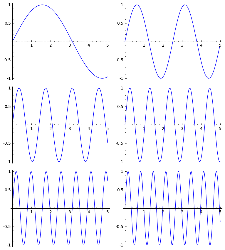
• interactive plots

• animations

• show and print

• solve command

Symbolic variables

Symbolic variables are similiar to regular variables. They can be defined using the command var. They are the building blocks of symbolic expressions.

var(x) defines a symbolic variable named x. (this is actually done for you by default when you start Sage. Be careful that you do not overwrite this symbolic variable with something else, like a number. You can get unexpected behavior if you are not careful.

DON'T DO THIS!

x = 5
plot(x^2) # plots a horizontal line at y = 25

var('x') 
(x*x^2 + cos(x)) # evaluates and simplifies expression

x x^3 + cos(x)

Symbolic Functions

These are different from regular python functions defined with the def keyword. Symbolic functions are one-command functions that take variables as arguments. This is probably best illustrated with some examples.

f(x) = 5*x^2
f

x |--> 5*x^2

See how f's representation is a function that takes one input and returns one output? Notice how the function's name is just f, not f(x).

We can plot f by using the plot command.

plot(f, (x,-3,3), figsize=4)

Interactive Plots

An interactive plot is used when you when to repeatedly try something, visualize your results, and change something again. To create an interactive plot, just put the decorator @interact over any regularly named function. The interactive plot will repeatedly evaluate your function with the arguments specified by the sliders/checkboxes.

REMEMBER! If you do not use the show or print command inside an interactive plot, no output will be displayed.

The syntax for the sliders is similar to srange: (start, end, step_size). If you want to have multiple sliders, just give your function multiple arguments. Leaving out the step size argument and just having two arguments makes the slider move continously.

In the example below, the m slider is continuous and the b slider goes in increments of 1.

@interact
def plot_a_function(m=(-3,3), b=(-5,5,1)):
    p = plot(m*x+b)
    show(p)

Interact: please open in CoCalc

You can also opt to just enter a number into a box. This is convenient if you don't know how fine of a resolution you need.

@interact
def change_a(a = 1): # lets you type in an answer; press enter to evaluate.
    p = plot(a*x^2+1)
    show(p)

Interact: please open in CoCalc

Animations

An animation is a sequence of figures played back in sequence. It is similar to how a flipbook or a movie works. Use the option gif=True to have it play back in a nice way for most browsers that won't take up too much bandwidth.

# sine with a decreasing period

blist = srange(1,10,.5)
list_of_plots = []
for b in blist:
    f(x) = sin(b*x)
    p = plot(f, (x,0,5), figsize=4)
    list_of_plots.append(p)
a = animate(list_of_plots)
show(a, gif=True) # need to show it in order to view it!

Show and Print

For the most part, show and print are almost exactly the same. You can think of show as being a "fancy print". Variables on their own line automatically get printed. Also worth noting is that if you want to view output or variables from inside a function or interactive, you'll need to explicitly use the print or show function to view the output.

# not that different here.
print(5)
show(5)

5

$\displaystyle 5$

# much more noticeable.
A = matrix([[1,2],[3,4]])
print(A)
show(A)

[1 2] [3 4]

$\displaystyle \left(\begin{array}{rr} 1 & 2 \\ 3 & 4 \end{array}\right)$

def no_output():
    a = 5
    a
no_output() # nothing printed

def show_output():
    b = 6
    print b
    show(b)
show_output() # prints, then shows the variable b

6

$\displaystyle 6$

The solve Command

The solve function is used for solving algebraic equations. While it can be used to find symbolic solutions to a single equation, it really shines when used to find solutions to systems of equations. This can be really helpful, for instance, in finding equilibrium points and in determining the number of solutions to a problem when searching for bifurcations. solve has a somewhat odd syntax and can be a bit clunky to use, but it is very powerful.

As a first example, we'll solve the equation $x^2 -3x + 2 = 0$.

Here is the function definition:

def solve(equations, variables_to_solve_for):

"equations" can be either a:

• single symbolic expression or a symbolic equation (something with ==)

• list of symbolic expressions or symbolic equations.

(We'll call a symbolic equation a symbolic expression that has a == in it. ) Symbolic expressions are automatically solved for when they are set equal to zero.

The variables_to_solve_for argument is either a:

• single symbolic variable to solve for

• list of symbolic variables to solve for These symbolic variables need to have been declared in advance.

# find root of single variable equation

var('x')

solve(x^2 -3*x + 2 == 0, x)
solve(x^2 -3*x + 2, x) # this does the exact same thing as the line above. Expressions are automatically equated to 0 if you don't specify anything else.
solve(x^2 -3*x + 2 ==2, x) # gets a different result

plot(x^2 -3*x + 2, (x,-1,4)) + plot(2, (x,-1,4), color= "red") + plot(0, (x,-1,4), color="green", thickness=3, figsize=4)

x [x == 1, x == 2] [x == 1, x == 2] [x == 0, x == 3]

We can either look at the output of the solve function very conveniently, but if we want to use the result of the calculation later on in your code, you will need to do a little bit more. As you can see, solve returns a list. You can access the solutions by indexing the list and calling the rhs() method on the result.

sol = solve(x^2 -3*x + 2 == 0, x)
sol[0].rhs() # gets the "right hand side" of the first solution
sol[1].rhs() # gets the same thing for the second solution
len(sol) # how many solutions there are.

1 2 2

If this syntax seems odd to you and/or you have multiple variables to deal with, you can use the keyword argument solution_dict=True to have the solution returned to you as a dict. Here is an example of solving a system of equations.

var('x')
var('y')

f = 2*x - y
g = -x -y

sol = solve([f == -1, g == 5], [x,y], solution_dict=True)
sol # sol is a list that has a dictionary for each solution. In this case, there is a single solution, (6,-11)
sol[0][x] # retrieve the value of x
sol[0][y] # retrieve the value of y

x y [{y: -3, x: -2}] -2 -3

We can plot these functions to verify that we have the correct solution. The solution is marked in red.

p = plot(2*x + 1, (x,-5,3)) + plot(-x-5, (x,-5,3)) + point([sol[0][x],sol[0][y]], color="red", size=40)
show(p, figsize=4)

Plotting points and text

Sagemath has built-in functionality for plotting text and points. Lines and boxes can also be found in the online documentation but are not covered here.

text("your text here", [3,4], axes_labels=['x','y']) # plotting a point at the coordinates (x=3, y=4)

# plotting points with varying sizes and colors. You can put the keyword arguments in any of the functions and they will apply to the entire graph.
point([5,2], size=50, color="red") + point([1,1], size=100, color="green") + point([2,5], axes_labels=['x','y'])

# plotting f(x) and marking f(2).

f(x) = 3*sin(x)

pt_coords = [2, f(2)]

my_text = "my_text"
text_coords = [2,f(2)+.5] # go up a little bit to avoid getting cut off by the function

plot(f, (x,0,5), axes_labels=['x','f(x)']) + point(coords, size=45) + text(my_text, text_coords)