2017-03-06.sagews

%md
# Math 152: Intro to Mathematical Software
### 2017-03-06
### Kiran Kedlaya; University of California, San Diego
### adapted from lectures by William Stein, University of Washington

### ** Lecture 23: SciPy: Additional tools for scientific computation **

Math 152: Intro to Mathematical Software

2017-03-06

Kiran Kedlaya; University of California, San Diego

adapted from lectures by William Stein, University of Washington

** Lecture 23: SciPy: Additional tools for scientific computation **

Announcements:

• This week's schedule is as usual: homework is due Tuesday at 8pm; peer review due Thursday at 8pm; sections and office hours meet as scheduled.

• However, next week's schedule will be modified because Peter and Zonglin and I will all be at a conference for part of the week.

  • The last homework will be due Friday, March 17 at 8pm. Peer review will be due Sunday, March 19 at 8pm.

  • Sections will not be held on Monday, March 13.

  • Office hours will be rescheduled for Thursday and Friday. The exact times will be announced later this week.

  • There will be guest lecturers on Monday and Wednesday. Details to be announced later.

• The window for course evaluations (CAPE) is open! Your detailed feedback will be greatly appreciated, and will help the math department with future course design.

Plan for the rest of the course:

• Today: finish the unit on scientific computation by demonstrating some additional functionality provide by SciPy. We will loosely follow the SciPy Tutorial.

• Rest of this week: abstract algebra and number theory.

• Next week: cryptography (including a preview of Math 187B, which will also use SageMathCloud).

Special functions

In addition to the basic functions you encounter in calculus (trig functions, exponential/logarithm), mathematicians have isolated a number of other special functions that occur from time to time, often when solving differential equations. See this list.

special.jn_zeros?

File: /projects/sage/sage-7.5/local/lib/python2.7/site-packages/scipy/special/basic.py
Signature : special.jn_zeros()
Docstring :
Compute zeros of integer-order Bessel function Jn(x).

n : int
   Order of Bessel function

nt : int
   Number of zeros to return

[1] Zhang, Shanjie and Jin, Jianming. "Computation of Special
    Functions", John Wiley and Sons, 1996, chapter 5.
    http://jin.ece.illinois.edu/specfunc.html

## Example: Bessel functions, used to calculate vibrational modes of a circular drum
%python
import numpy as np
from scipy import special

def drumhead_height(n, k, distance, angle, t):
   kth_zero = special.jn_zeros(n, k)[-1]
   return np.cos(t) * np.cos(n*angle) * special.jn(n, distance*kth_zero)
theta = np.r_[0:2*np.pi:50j]
radius = np.r_[0:1:50j]
x = np.array([r * np.cos(theta) for r in radius])
y = np.array([r * np.sin(theta) for r in radius])
z = np.array([drumhead_height(3, 1, r, theta, 0.5) for r in radius])

import matplotlib.pyplot as plt
from mpl_toolkits.mplot3d import Axes3D
from matplotlib import cm
fig = plt.figure()
ax = Axes3D(fig)
ax.plot_surface(x, y, z, rstride=1, cstride=1, cmap=cm.jet)
ax.set_xlabel('X')
ax.set_ylabel('Y')
ax.set_zlabel('Z')
plt.show()

<mpl_toolkits.mplot3d.art3d.Poly3DCollection object at 0x7fa9ec9827d0> <matplotlib.text.Text object at 0x7fa9ec985b90> <matplotlib.text.Text object at 0x7fa9e6e096d0> <matplotlib.text.Text object at 0x7fa9e6d47a50>

## The error function, i.e., the integral of a Gaussian normal distribution.
x = np.linspace(-3, 3)
plt.plot(x, special.erf(x))
plt.xlabel('$x$')
plt.ylabel('$erf(x)$')
plt.show()

[<matplotlib.lines.Line2D object at 0x7fa9e6b03590>] <matplotlib.text.Text object at 0x7fa9ec9bbb10> <matplotlib.text.Text object at 0x7fa9ec9d6750>

## This one is available in Sage also.
plot(erf, (-3,3))

Integration

In case you need something more sophisticated than Sage's built-in numerical integration, some options can be found here. Here I'll demonstrate one example: numerically solving an ordinary differential equation (ODE).

Consider the second-order equation [\frac{d^{2}w}{dz^{2}}-zw(z)=0] with initial conditions (w\left(0\right)=\frac{1}{\sqrt[3]{3^{2}}\Gamma\left(\frac{2}{3}\right)}) and (\left.\frac{dw}{dz}\right|_{z=0}=-\frac{1}{\sqrt[3]{3}\Gamma\left(\frac{1}{3}\right)}.) It is known that the solution to this differential equation with these boundary conditions is the Airy function [w=\textrm{Ai}\left(z\right);] let us compare the numerical result against the SciPy function special.airy.

To use the SciPy solve, we must first convert this ODE into a first-order system by setting (\mathbf{y}=\left[\frac{dw}{dz},w\right]) and (t=z). Thus, the differential equation becomes [$$\begin{split}\frac{d\mathbf{y}}{dt}=\left[\begin{array}{c} ty_{1}\\ y_{0}\end{array}\right]=\left[\begin{array}{cc} 0 & t\\ 1 & 0\end{array}\right]\left[\begin{array}{c} y_{0}\\ y_{1}\end{array}\right]=\left[\begin{array}{cc} 0 & t\\ 1 & 0\end{array}\right]\mathbf{y}.\end{split}$$]

In other words, [\mathbf{f}\left(\mathbf{y},t\right)=\mathbf{A}\left(t\right)\mathbf{y}.]

The required inputs to odeint are the function defining the derivative, fprime; the initial conditions vector, y0; and the evaluation points at which to obtain a solution, t (with the initial value point as the first element of this sequence). The output is a matrix where each row contains the solution vector at each requested evaluation point (the initial conditions are given in the first output row).

%python3
from scipy.integrate import odeint
from scipy.special import gamma, airy
y1_0 = 1.0 / 3**(2.0/3.0) / gamma(2.0/3.0)
y0_0 = -1.0 / 3**(1.0/3.0) / gamma(1.0/3.0)
y0 = [y0_0, y1_0]
def func(y, t):
    return [t*y[1],y[0]]

def gradient(y, t):
    return [[0,t], [1,0]]

x = np.arange(0, 4.0, 0.01)
t = x
ychk = airy(x)[0]
y = odeint(func, y0, t)
y2 = odeint(func, y0, t, Dfun=gradient)

ychk[:36:6] ## values computed using the built-in Airy function

array([ 0.35502805, 0.33951139, 0.32406751, 0.30876307, 0.29365818, 0.27880648])

%python3
import matplotlib.pyplot as plt
plt.figure()
plt.plot(x, y[:, 1])
plt.show()

y[:36:6,1] ## values computed using odeint

array([ 0.35502805, 0.33951138, 0.32406749, 0.30876306, 0.29365817, 0.27880648])

y2[:36:6,1] ## values computed using odeint with user-specified gradient

array([ 0.35502805, 0.33951138, 0.32406749, 0.30876306, 0.29365817, 0.27880648])

odeint?

File: /projects/sage/sage-7.5/local/lib/python2.7/site-packages/scipy/integrate/odepack.py
Signature : odeint(func, y0, t, args=(), Dfun=None, col_deriv=0, full_output=0, ml=None, mu=None, rtol=None, atol=None, tcrit=None, h0=0.0, hmax=0.0, hmin=0.0, ixpr=0, mxstep=0, mxhnil=0, mxordn=12, mxords=5, printmessg=0)
Docstring :
Integrate a system of ordinary differential equations.

Solve a system of ordinary differential equations using lsoda from
the FORTRAN library odepack.

Solves the initial value problem for stiff or non-stiff systems of
first order ode-s:

   dy/dt = func(y, t0, ...)

where y can be a vector.

*Note*: The first two arguments of "func(y, t0, ...)" are in the
opposite order of the arguments in the system definition function
used by the scipy.integrate.ode class.

func : callable(y, t0, ...)
   Computes the derivative of y at t0.

y0 : array
   Initial condition on y (can be a vector).

t : array
   A sequence of time points for which to solve for y.  The initial
   value point should be the first element of this sequence.

args : tuple, optional
   Extra arguments to pass to function.

Dfun : callable(y, t0, ...)
   Gradient (Jacobian) of func.

col_deriv : bool, optional
   True if Dfun defines derivatives down columns (faster),
   otherwise Dfun should define derivatives across rows.

full_output : bool, optional
   True if to return a dictionary of optional outputs as the second
   output

printmessg : bool, optional
   Whether to print the convergence message

y : array, shape (len(t), len(y0))
   Array containing the value of y for each desired time in t, with
   the initial value y0 in the first row.

infodict : dict, only returned if full_output == True
   Dictionary containing additional output information

   +---------+--------------------------------------------------------------+
   | key     | meaning                                                      |
   +=========+==============================================================+
   | 'hu'    | vector of step sizes successfully used for each time step.   |
   +---------+--------------------------------------------------------------+
   | 'tcur'  | vector with the value of t reached for each time step. (will |
   |         | always be at least as large as the input times).             |
   +---------+--------------------------------------------------------------+
   | 'tolsf' | vector of tolerance scale factors, greater than 1.0,         |
   |         | computed when a request for too much accuracy was detected.  |
   +---------+--------------------------------------------------------------+
   | 'tsw'   | value of t at the time of the last method switch (given for  |
   |         | each time step)                                              |
   +---------+--------------------------------------------------------------+
   | 'nst'   | cumulative number of time steps                              |
   +---------+--------------------------------------------------------------+
   | 'nfe'   | cumulative number of function evaluations for each time step |
   +---------+--------------------------------------------------------------+
   | 'nje'   | cumulative number of jacobian evaluations for each time step |
   +---------+--------------------------------------------------------------+
   | 'nqu'   | a vector of method orders for each successful step.          |
   +---------+--------------------------------------------------------------+
   | 'imxer' | index of the component of largest magnitude in the weighted  |
   |         | local error vector (e / ewt) on an error return, -1          |
   |         | otherwise.                                                   |
   +---------+--------------------------------------------------------------+
   | 'lenrw' | the length of the double work array required.                |
   +---------+--------------------------------------------------------------+
   | 'leniw' | the length of integer work array required.                   |
   +---------+--------------------------------------------------------------+
   | 'mused' | a vector of method indicators for each successful time step: |
   |         | 1: adams (nonstiff), 2: bdf (stiff)                          |
   +---------+--------------------------------------------------------------+

ml, mu : int, optional
   If either of these are not None or non-negative, then the
   Jacobian is assumed to be banded.  These give the number of
   lower and upper non-zero diagonals in this banded matrix. For
   the banded case, Dfun should return a matrix whose rows contain
   the non-zero bands (starting with the lowest diagonal). Thus,
   the return matrix jac from Dfun should have shape "(ml + mu + 1,
   len(y0))" when "ml >=0" or "mu >=0". The data in jac must be
   stored such that "jac[i - j + mu, j]" holds the derivative of
   the i`th equation with respect to the `j`th state variable.  If
   `col_deriv is True, the transpose of this jac must be returned.

rtol, atol : float, optional
   The input parameters rtol and atol determine the error control
   performed by the solver.  The solver will control the vector, e,
   of estimated local errors in y, according to an inequality of
   the form "max-norm of (e / ewt) <= 1", where ewt is a vector of
   positive error weights computed as "ewt = rtol * abs(y) + atol".
   rtol and atol can be either vectors the same length as y or
   scalars. Defaults to 1.49012e-8.

tcrit : ndarray, optional
   Vector of critical points (e.g. singularities) where integration
   care should be taken.

h0 : float, (0: solver-determined), optional
   The step size to be attempted on the first step.

hmax : float, (0: solver-determined), optional
   The maximum absolute step size allowed.

hmin : float, (0: solver-determined), optional
   The minimum absolute step size allowed.

ixpr : bool, optional
   Whether to generate extra printing at method switches.

mxstep : int, (0: solver-determined), optional
   Maximum number of (internally defined) steps allowed for each
   integration point in t.

mxhnil : int, (0: solver-determined), optional
   Maximum number of messages printed.

mxordn : int, (0: solver-determined), optional
   Maximum order to be allowed for the non-stiff (Adams) method.

mxords : int, (0: solver-determined), optional
   Maximum order to be allowed for the stiff (BDF) method.

ode : a more object-oriented integrator based on VODE. quad : for
finding the area under a curve.

The second order differential equation for the angle theta of a
pendulum acted on by gravity with friction can be written:

   theta''(t) + b*theta'(t) + c*sin(theta(t)) = 0

where b and c are positive constants, and a prime (') denotes a
derivative.  To solve this equation with odeint, we must first
convert it to a system of first order equations.  By defining the
angular velocity "omega(t) = theta'(t)", we obtain the system:

   theta'(t) = omega(t)
   omega'(t) = -b*omega(t) - c*sin(theta(t))

Let y be the vector [theta, omega].  We implement this system in
python as:

>>> def pend(y, t, b, c):
...     theta, omega = y
...     dydt = [omega, -b*omega - c*np.sin(theta)]
...     return dydt
...

We assume the constants are b = 0.25 and c = 5.0:

>>> b = 0.25
>>> c = 5.0

For initial conditions, we assume the pendulum is nearly vertical
with theta(0) = pi - 0.1, and it initially at rest, so omega(0) =
0.  Then the vector of initial conditions is

>>> y0 = [np.pi - 0.1, 0.0]

We generate a solution 101 evenly spaced samples in the interval 0
<= t <= 10.  So our array of times is:

>>> t = np.linspace(0, 10, 101)

Call odeint to generate the solution.  To pass the parameters b and
c to pend, we give them to odeint using the args argument.

>>> from scipy.integrate import odeint
>>> sol = odeint(pend, y0, t, args=(b, c))

The solution is an array with shape (101, 2).  The first column is
theta(t), and the second is omega(t).  The following code plots
both components.

>>> import matplotlib.pyplot as plt
>>> plt.plot(t, sol[:, 0], 'b', label='theta(t)')
>>> plt.plot(t, sol[:, 1], 'g', label='omega(t)')
>>> plt.legend(loc='best')
>>> plt.xlabel('t')
>>> plt.grid()
>>> plt.show()

## What if we use the wrong gradient?

def gradient2(y, t):
    return [[0,t^2-t-1], [1,-t]]

y2 = odeint(func, y0, t, Dfun=gradient2)

y2[:36:6,1] ## Appears to affect the runtime, but not the solution.

array([ 0.35502805, 0.33951138, 0.32406749, 0.30876306, 0.29365817, 0.27880648])

Fourier transforms

A one-dimensional discrete Fourier transform:

The FFT y[k] of length (N) of the length-(N) sequence $x[n]$ is defined as [y[k] = \sum_{n=0}^{N-1} e^{-2 \pi j \frac{k n}{N} } x[n] , ,] and the inverse transform is defined as [x[n] = \frac{1}{N} \sum_{n=0}^{N-1} e^{2 \pi j \frac{k n}{N} } y[k] , .]

These transforms can be calculated by means of fft and ifft, respectively.

from scipy.fftpack import fft, ifft
x = np.array([1.0, 2.0, 1.0, -1.0, 1.5])
y = fft(x)
y

array([ 4.50000000+0.j , 2.08155948-1.65109876j, -1.83155948+1.60822041j, -1.83155948-1.60822041j, 2.08155948+1.65109876j])

yinv = ifft(y)
yinv

array([ 1.0+0.j, 2.0+0.j, 1.0+0.j, -1.0+0.j, 1.5+0.j])

Consistency check: from the definitions, we must have [y[0] = \sum_{n=0}^{N-1} x[n] , .]

x.sum(), y[0]

(4.5, (4.5+0j))

y.sum(), x[0]

((5+0j), 1.0)

One typical reason to perform a Fourier transform is to pick out periodic contributions to a signal (i.e., frequencies). Let's try this with a sum of two sine functions.

from scipy.fftpack import fft
# Number of sample points
N = 6000
# sample spacing
T = 1.0 / 800.0
x = np.linspace(0.0, N*T, N)
y = np.sin(50.0 * 2.0*np.pi*x) + 0.5*np.sin(80.0 * 2.0*np.pi*x)
yf = fft(y)

xf = np.linspace(0.0, 1.0/(2.0*T), N/2)
import matplotlib.pyplot as plt
plt.plot(xf, 2.0/N * np.abs(yf[0:N/2]))
plt.grid()
plt.show()

[<matplotlib.lines.Line2D object at 0x7fa9e2e73ad0>]

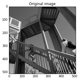
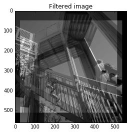
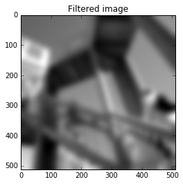
Signal processing: filters

Here the basic ideal is that you have a "signal" consisting of a large array of numbers, but you only want to retain a smaller array that captures most of the essential information. A typical example is image processing. (The Snap IPO suggests there is big money in this!)

File: /projects/sage/sage-7.5/local/lib/python2.7/site-packages/scipy/misc/common.py
Signature : misc.lena()
Docstring :
Function that previously returned an example image

Note: Removed in 0.17

None

None

RuntimeError
   This functionality has been removed due to licensing reasons.

The image previously returned by this function has an incompatible
license and has been removed from SciPy. Please use face or ascent
instead.

face, ascent

%python3 # This seems to work better in python3, not sure why.
from scipy import signal, misc
import matplotlib.pyplot as plt

image = misc.ascent()
plt.figure()
plt.imshow(image)
plt.gray()
plt.title('Original image')
plt.show()

%python3
import numpy as np

w = np.zeros((50, 50))
w[0][0] = 1.0
w[49][25] = 1.0
image_new = signal.fftconvolve(image, w)

plt.figure()
plt.imshow(image_new)
plt.gray()
plt.title('Filtered image')
plt.show()

%python3
w = signal.gaussian(50, 10.0)
image_new = signal.sepfir2d(image, w, w)

plt.figure()
plt.imshow(image_new)
plt.gray()
plt.title('Filtered image')
plt.show()

%python3
image_new2 = signal.wiener(image_new)

plt.figure()
plt.imshow(image_new2)
plt.gray()
plt.title('Filtered image')
plt.show()