Contact
CoCalc Logo Icon
StoreFeaturesDocsShareSupport News AboutSign UpSign In
| Download
Views: 16658
%md # Math 152: Intro to Mathematical Software ### 2017-02-17 ### Kiran Kedlaya; University of California, San Diego ### adapted from lectures by William Stein, University of Washington <img src="http://blogs.sandiegozoo.org/wp-content/uploads/2013/08/PandaCubGrowthCurve-25Jul13.jpg" class="pull-right" width=300> ### ** Lecture 17: Pandas (part 3): Statistics **

Math 152: Intro to Mathematical Software

2017-02-17

Kiran Kedlaya; University of California, San Diego

adapted from lectures by William Stein, University of Washington
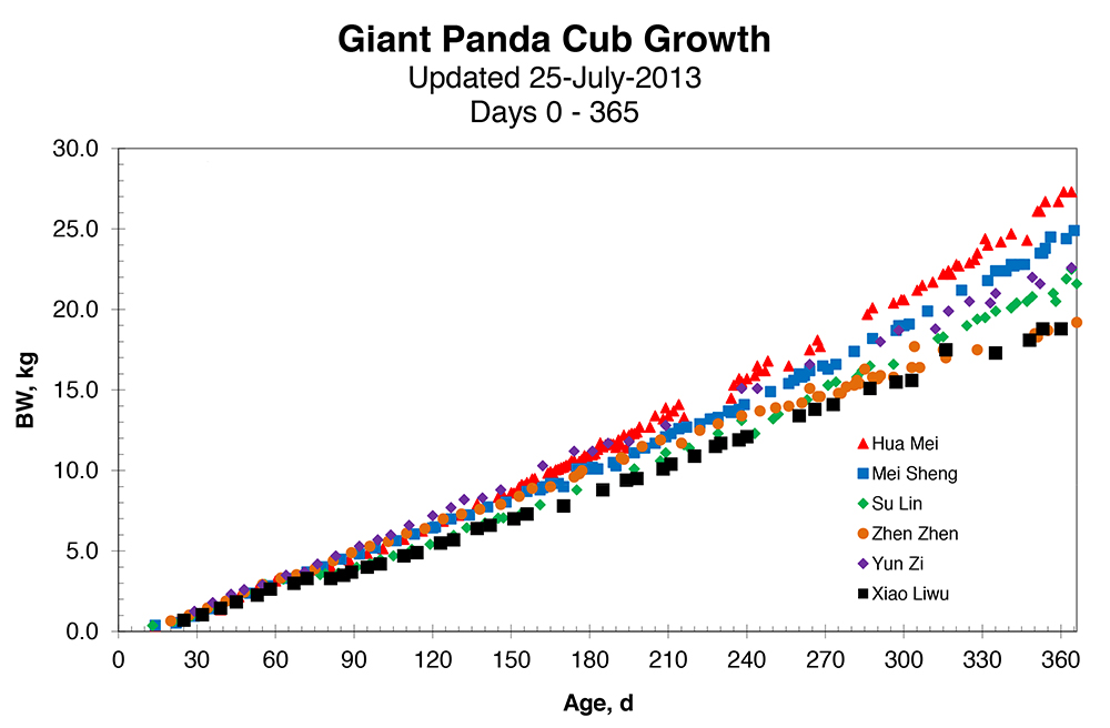
** Lecture 17: Pandas (part 3): Statistics **

Today's topics:

  • statsmodels

  • scikit-learn

Here's a slideshow about the "data analysis and statistics in python", with comparisons to R. (You can also run R in a worksheet using %R, but I am not a statistician so I won't be able to offer much assistance with that.)

statsmodels

"Python module that allows users to explore data, estimate statistical models, and perform statistical tests."

Documentation: http://statsmodels.sourceforge.net/stable/

%auto %default_mode python %typeset_mode True import statsmodels.api as sm import pandas from patsy import dmatrices
/ext/sage/sage-8.1/local/lib/python2.7/site-packages/statsmodels/compat/pandas.py:56: FutureWarning: The pandas.core.datetools module is deprecated and will be removed in a future version. Please use the pandas.tseries module instead. from pandas.core import datetools

1. The statsmodels "Getting started" tutorial!

We download the Guerry dataset, a collection of historical data used in support of Andre-Michel Guerry’s 1833 Essay on the Moral Statistics of France. The data set is hosted online in comma-separated values format (CSV) by the Rdatasets repository. We could download the file locally and then load it using read_csv, but pandas takes care of all of this automatically for us:

df = sm.datasets.get_rdataset("Guerry", "HistData").data # this is a familiar Pandas dataframe df.head()
dept Region Department Crime_pers Crime_prop Literacy Donations Infants Suicides MainCity Wealth Commerce Clergy Crime_parents Infanticide Donation_clergy Lottery Desertion Instruction Prostitutes Distance Area Pop1831
0 1 E Ain 28870 15890 37 5098 33120 35039 2:Med 73 58 11 71 60 69 41 55 46 13 218.372 5762 346.03
1 2 N Aisne 26226 5521 51 8901 14572 12831 2:Med 22 10 82 4 82 36 38 82 24 327 65.945 7369 513.00
2 3 C Allier 26747 7925 13 10973 17044 114121 2:Med 61 66 68 46 42 76 66 16 85 34 161.927 7340 298.26
3 4 E Basses-Alpes 12935 7289 46 2733 23018 14238 1:Sm 76 49 5 70 12 37 80 32 29 2 351.399 6925 155.90
4 5 E Hautes-Alpes 17488 8174 69 6962 23076 16171 1:Sm 83 65 10 22 23 64 79 35 7 1 320.280 5549 129.10

We select the variables of interest and look at the bottom 5 rows:

df = df[ ['Department', 'Lottery', 'Literacy', 'Wealth', 'Region'] ] df.tail(5)
Department Lottery Literacy Wealth Region
81 Vienne 40 25 68 W
82 Haute-Vienne 55 13 67 C
83 Vosges 14 62 82 E
84 Yonne 51 47 30 C
85 Corse 83 49 37 NaN

Notice that there is one missing observation in the Region column. We eliminate it using a DataFrame method provided by pandas:

df = df.dropna() df.tail(5)
Department Lottery Literacy Wealth Region
80 Vendee 68 28 56 W
81 Vienne 40 25 68 W
82 Haute-Vienne 55 13 67 C
83 Vosges 14 62 82 E
84 Yonne 51 47 30 C

Some statistics...

Substantive motivation and model: We want to know whether literacy rates in the 86 French departments are associated with per capita wagers on the Royal Lottery in the 1820s. We need to control for the level of wealth in each department, and we also want to include a series of dummy variables on the right-hand side of our regression equation to control for unobserved heterogeneity due to regional effects. The model is estimated using ordinary least squares regression (OLS).

(WARNING: I'm not a statistician...)

Use patsy‘s to create design matrices, then use statsmodels to do an ordinary least squares fit.

y,X = dmatrices('Lottery ~ Literacy + Wealth + Region', data=df, return_type='dataframe') mod = sm.OLS(y, X) # Describe model res = mod.fit() # Fit model res.summary() # Summarize model
/projects/sage/sage-7.5/local/lib/python2.7/site-packages/patsy/util.py:652: DeprecationWarning: pandas.core.common.is_categorical_dtype is deprecated. import from the public API: pandas.api.types.is_categorical_dtype instead return safe_is_pandas_categorical_dtype(data.dtype) /projects/sage/sage-7.5/local/lib/python2.7/site-packages/patsy/util.py:679: DeprecationWarning: pandas.core.common.is_categorical_dtype is deprecated. import from the public API: pandas.api.types.is_categorical_dtype instead if safe_is_pandas_categorical_dtype(dt1):
OLS Regression Results ============================================================================== Dep. Variable: Lottery R-squared: 0.338 Model: OLS Adj. R-squared: 0.287 Method: Least Squares F-statistic: 6.636 Date: Fri, 17 Feb 2017 Prob (F-statistic): 1.07e-05 Time: 22:12:49 Log-Likelihood: -375.30 No. Observations: 85 AIC: 764.6 Df Residuals: 78 BIC: 781.7 Df Model: 6 Covariance Type: nonrobust =============================================================================== coef std err t P>|t| [95.0% Conf. Int.] ------------------------------------------------------------------------------- Intercept 38.6517 9.456 4.087 0.000 19.826 57.478 Region[T.E] -15.4278 9.727 -1.586 0.117 -34.793 3.938 Region[T.N] -10.0170 9.260 -1.082 0.283 -28.453 8.419 Region[T.S] -4.5483 7.279 -0.625 0.534 -19.039 9.943 Region[T.W] -10.0913 7.196 -1.402 0.165 -24.418 4.235 Literacy -0.1858 0.210 -0.886 0.378 -0.603 0.232 Wealth 0.4515 0.103 4.390 0.000 0.247 0.656 ============================================================================== Omnibus: 3.049 Durbin-Watson: 1.785 Prob(Omnibus): 0.218 Jarque-Bera (JB): 2.694 Skew: -0.340 Prob(JB): 0.260 Kurtosis: 2.454 Cond. No. 371. ============================================================================== Warnings: [1] Standard Errors assume that the covariance matrix of the errors is correctly specified.

statsmodels also provides graphics functions. For example, we can draw a plot of partial regression for a set of regressors by:

sm.graphics.plot_partregress?
File: /projects/sage/sage-7.5/local/lib/python2.7/site-packages/statsmodels/graphics/regressionplots.py Signature : sm.graphics.plot_partregress(endog, exog_i, exog_others, data=None, title_kwargs={}, obs_labels=True, label_kwargs={}, ax=None, ret_coords=False, **kwds) Docstring : Plot partial regression for a single regressor. endog : ndarray or string endogenous or response variable. If string is given, you can use a arbitrary translations as with a formula. exog_i : ndarray or string exogenous, explanatory variable. If string is given, you can use a arbitrary translations as with a formula. exog_others : ndarray or list of strings other exogenous, explanatory variables. If a list of strings is given, each item is a term in formula. You can use a arbitrary translations as with a formula. The effect of these variables will be removed by OLS regression. data : DataFrame, dict, or recarray Some kind of data structure with names if the other variables are given as strings. title_kwargs : dict Keyword arguments to pass on for the title. The key to control the fonts is fontdict. obs_labels : bool or array-like Whether or not to annotate the plot points with their observation labels. If obs_labels is a boolean, the point labels will try to do the right thing. First it will try to use the index of data, then fall back to the index of exog_i. Alternatively, you may give an array-like object corresponding to the obseveration numbers. labels_kwargs : dict Keyword arguments that control annotate for the observation labels. ax : Matplotlib AxesSubplot instance, optional If given, this subplot is used to plot in instead of a new figure being created. ret_coords : bool If True will return the coordinates of the points in the plot. You can use this to add your own annotations. kwargs The keyword arguments passed to plot for the points. fig : Matplotlib figure instance If ax is None, the created figure. Otherwise the figure to which ax is connected. coords : list, optional If ret_coords is True, return a tuple of arrays (x_coords, y_coords). The slope of the fitted line is the that of exog_i in the full multiple regression. The individual points can be used to assess the influence of points on the estimated coefficient. plot_partregress_grid : Plot partial regression for a set of regressors.
sm.graphics.plot_partregress('Lottery', 'Wealth', ['Region', 'Literacy'], data=df, obs_labels=False)

2. Scikit Learn: Easy Machine Learning

From their website:

Machine Learning in Python

  • Simple and efficient tools for data mining and data analysis

  • Accessible to everybody, and reusable in various contexts

  • Built on NumPy, SciPy, and matplotlib

  • Open source, commercially usable - BSD license

from sklearn import datasets digits = datasets.load_digits()

This "digits" thing is 1797 hand-written low-resolution numbers from the postal code numbers on letters (zip codes)...

type(digits.data)
<type 'numpy.ndarray'>
digits.data
[[ 0. 0. 5. ..., 0. 0. 0.] [ 0. 0. 0. ..., 10. 0. 0.] [ 0. 0. 0. ..., 16. 9. 0.] ..., [ 0. 0. 1. ..., 6. 0. 0.] [ 0. 0. 2. ..., 12. 0. 0.] [ 0. 0. 10. ..., 12. 1. 0.]]
digits.target
[0 1 2 ..., 8 9 8]
digits.images[200], digits.target[200]
[[ 0. 0. 0. 0. 11. 12. 0. 0.] [ 0. 0. 0. 3. 15. 14. 0. 0.] [ 0. 0. 0. 11. 16. 11. 0. 0.] [ 0. 0. 9. 16. 16. 10. 0. 0.] [ 0. 4. 16. 12. 16. 12. 0. 0.] [ 0. 3. 10. 3. 16. 11. 0. 0.] [ 0. 0. 0. 0. 16. 14. 0. 0.] [ 0. 0. 0. 0. 11. 11. 0. 0.]]
(1\displaystyle 1)
len(digits.target)
1797\displaystyle 1797
import matplotlib.pyplot as plt def plot_data(n): print "scan of %s"%digits.target[n] show(plt.matshow(digits.data[n].reshape(8,8), interpolation="nearest", cmap=plt.cm.Greys_r))
digits.images[0]
[[ 0. 0. 5. 13. 9. 1. 0. 0.] [ 0. 0. 13. 15. 10. 15. 5. 0.] [ 0. 3. 15. 2. 0. 11. 8. 0.] [ 0. 4. 12. 0. 0. 8. 8. 0.] [ 0. 5. 8. 0. 0. 9. 8. 0.] [ 0. 4. 11. 0. 1. 12. 7. 0.] [ 0. 2. 14. 5. 10. 12. 0. 0.] [ 0. 0. 6. 13. 10. 0. 0. 0.]]
digits.data[0]
[ 0. 0. 5. 13. 9. 1. 0. 0. 0. 0. 13. 15. 10. 15. 5. 0. 0. 3. 15. 2. 0. 11. 8. 0. 0. 4. 12. 0. 0. 8. 8. 0. 0. 5. 8. 0. 0. 9. 8. 0. 0. 4. 11. 0. 1. 12. 7. 0. 0. 2. 14. 5. 10. 12. 0. 0. 0. 0. 6. 13. 10. 0. 0. 0.]
plot_data(200)
scan of 1
plot_data(389) digits.target[389]
scan of 3
3\displaystyle 3

Example/goal here:

"In the case of the digits dataset, the task is to predict, given an image, which digit it represents. We are given 1797 samples of each of the 10 possible classes (the digits zero through nine) on which we fit an estimator to be able to predict the classes to which unseen samples belong."

from sklearn import svm # use a support vector machine... clf = svm.SVC(gamma=0.001, C=100.) # We set params manually;, but scikit learn has techniques for finding these params automatically
plot_data(1796)
scan of 8

This clf is a "classifier". Right now it doesn't know anything at all about our actual data.

We teach it by passing in our data to the fit method...

"We use all the images of our dataset apart from the last one. We select this training set with the [:-1] Python syntax, which produces a new array that contains all but the last entry of digits.data:"

# Train our classifier by giving it 1796 scanned digits! clf.fit(digits.data[:-2], digits.target[:-2])
SVC(C=100.0, cache_size=200, class_weight=None, coef0=0.0, decision_function_shape=None, degree=3, gamma=0.001, kernel='rbf', max_iter=-1, probability=False, random_state=None, shrinking=True, tol=0.001, verbose=False)
plot_data(1796) # the last one -- not given
scan of 8
digits.data[-1:]
[[ 0. 0. 10. 14. 8. 1. 0. 0. 0. 2. 16. 14. 6. 1. 0. 0. 0. 0. 15. 15. 8. 15. 0. 0. 0. 0. 5. 16. 16. 10. 0. 0. 0. 0. 12. 15. 15. 12. 0. 0. 0. 4. 16. 6. 4. 16. 6. 0. 0. 8. 16. 10. 8. 16. 8. 0. 0. 1. 8. 12. 14. 12. 1. 0.]]
digits.target[-2:]
[9 8]
# it predicts it is an 8 correctly! clf.predict(digits.data[-2:])
[9 8]

** Exercise for you right now: ** Run the prediction on all 1797 scanned values to see how many are correct.

# To get you started, here is how to test the 5 scanned value. digits.target[5] clf.predict(digits.data[5:6])
5\displaystyle 5
[5]
n = 15 digits.target[n] == clf.predict(digits.data[n:n+1])[0]
True
# After you do this -- completely recreate clf but trained on way less data!
clf.fit(digits.data[:1000], digits.target[:1000]) pre = clf.predict(digits.data[1000:]) ans = digits.target[1000:]
SVC(C=100.0, cache_size=200, class_weight=None, coef0=0.0, decision_function_shape=None, degree=3, gamma=0.001, kernel='rbf', max_iter=-1, probability=False, random_state=None, shrinking=True, tol=0.001, verbose=False)
len([i for i in range(797) if pre[i] == ans[i]])
773\displaystyle 773
plot_data(5)
scan of 5

bonus

plots of low dimensional embeddings of the digits dataset:

http://scikit-learn.org/stable/auto_examples/manifold/plot_lle_digits.html