| Download

Project: ⛏️ hsy development

Path: examples/bayesian-methods-for-hackers / Chapter4_TheGreatestTheoremNeverTold / Ch4_LawOfLargeNumbers_TFP.ipynb

Views: ³¹⁹⁴

Kernel: Python 3

Probabilistic Programming and Bayesian Methods for Hackers Chapter 4

Run in Google Colab

View source on GitHub

Original content (this Jupyter notebook) created by Cam Davidson-Pilon (@Cmrn_DP)

Ported to Tensorflow Probability by Matthew McAteer (@MatthewMcAteer0), with help from the TFP team at Google ([email protected]).

Welcome to Bayesian Methods for Hackers. The full Github repository is available at github/Probabilistic-Programming-and-Bayesian-Methods-for-Hackers. The other chapters can be found on the project's homepage. We hope you enjoy the book, and we encourage any contributions!

Dependencies & Prerequisites
The greatest theorem never told
- The Law of Large Numbers
- Intuition
- How do we compute $Var(Z)$ though?
- Expected values and probabilities
- What does this all have to do with Bayesian statistics?
- The Disorder of Small Numbers
- Example: Aggregated geographic data
- Example: Kaggle's U.S. Census Return Rate Challenge
- Example: How to order Reddit submissions
  - Setting up the Praw Reddit API
  - Register your Application on Reddit
    - Reddit API Setup
  - Sorting!
  - But this is too slow for real-time!
- Extension to Starred rating systems
- Example: Counting Github stars
- Conclusion
- Appendix
  - Exercises
  - Kicker Careers Ranked by Make Percentage
  - Average Household Income by Programming Language
- References

Dependencies & Prerequisites

Tensorflow Probability is part of the colab default runtime, so you don't need to install Tensorflow or Tensorflow Probability if you're running this in the colab.
If you're running this notebook in Jupyter on your own machine (and you have already installed Tensorflow), you can use the following

For the most recent nightly installation: pip3 install -q tfp-nightly
For the most recent stable TFP release: pip3 install -q --upgrade tensorflow-probability
For the most recent stable GPU-connected version of TFP: pip3 install -q --upgrade tensorflow-probability-gpu
For the most recent nightly GPU-connected version of TFP: pip3 install -q tfp-nightly-gpu

Again, if you are running this in a Colab, Tensorflow and TFP are already installed

In [1]:

#@title Imports and Global Variables  { display-mode: "form" }
"""
The book uses a custom matplotlibrc file, which provides the unique styles for
matplotlib plots. If executing this book, and you wish to use the book's
styling, provided are two options:
    1. Overwrite your own matplotlibrc file with the rc-file provided in the
       book's styles/ dir. See http://matplotlib.org/users/customizing.html
    2. Also in the styles is  bmh_matplotlibrc.json file. This can be used to
       update the styles in only this notebook. Try running the following code:

        import json
        s = json.load(open("../styles/bmh_matplotlibrc.json"))
        matplotlib.rcParams.update(s)
"""
!pip3 install -q praw
!pip3 install -q pandas_datareader
!pip3 install -q wget
from __future__ import absolute_import, division, print_function

#@markdown This sets the warning status (default is `ignore`, since this notebook runs correctly)
warning_status = "ignore" #@param ["ignore", "always", "module", "once", "default", "error"]
import warnings
warnings.filterwarnings(warning_status)
with warnings.catch_warnings():
    warnings.filterwarnings(warning_status, category=DeprecationWarning)
    warnings.filterwarnings(warning_status, category=UserWarning)

import numpy as np
import os
#@markdown This sets the styles of the plotting (default is styled like plots from [FiveThirtyeight.com](https://fivethirtyeight.com/))
matplotlib_style = 'fivethirtyeight' #@param ['fivethirtyeight', 'bmh', 'ggplot', 'seaborn', 'default', 'Solarize_Light2', 'classic', 'dark_background', 'seaborn-colorblind', 'seaborn-notebook']
import matplotlib.pyplot as plt; plt.style.use(matplotlib_style)
import matplotlib.axes as axes;
from matplotlib.patches import Ellipse
from mpl_toolkits.mplot3d import Axes3D
import pandas_datareader.data as web
%matplotlib inline
import seaborn as sns; sns.set_context('notebook')
from IPython.core.pylabtools import figsize
#@markdown This sets the resolution of the plot outputs (`retina` is the highest resolution)
notebook_screen_res = 'retina' #@param ['retina', 'png', 'jpeg', 'svg', 'pdf']
%config InlineBackend.figure_format = notebook_screen_res

import tensorflow as tf
tfe = tf.contrib.eager

# Eager Execution
#@markdown Check the box below if you want to use [Eager Execution](https://www.tensorflow.org/guide/eager)
#@markdown Eager execution provides An intuitive interface, Easier debugging, and a control flow comparable to Numpy. You can read more about it on the [Google AI Blog](https://ai.googleblog.com/2017/10/eager-execution-imperative-define-by.html)
use_tf_eager = False #@param {type:"boolean"}

# Use try/except so we can easily re-execute the whole notebook.
if use_tf_eager:
    try:
        tf.enable_eager_execution()
    except:
        pass

import tensorflow_probability as tfp
tfd = tfp.distributions
tfb = tfp.bijectors

  
def evaluate(tensors):
    """Evaluates Tensor or EagerTensor to Numpy `ndarray`s.
    Args:
    tensors: Object of `Tensor` or EagerTensor`s; can be `list`, `tuple`,
      `namedtuple` or combinations thereof.
   
    Returns:
      ndarrays: Object with same structure as `tensors` except with `Tensor` or
        `EagerTensor`s replaced by Numpy `ndarray`s.
    """
    if tf.executing_eagerly():
        return tf.contrib.framework.nest.pack_sequence_as(
            tensors,
            [t.numpy() if tf.contrib.framework.is_tensor(t) else t
             for t in tf.contrib.framework.nest.flatten(tensors)])
    return sess.run(tensors)

class _TFColor(object):
    """Enum of colors used in TF docs."""
    red = '#F15854'
    blue = '#5DA5DA'
    orange = '#FAA43A'
    green = '#60BD68'
    pink = '#F17CB0'
    brown = '#B2912F'
    purple = '#B276B2'
    yellow = '#DECF3F'
    gray = '#4D4D4D'
    def __getitem__(self, i):
        return [
            self.red,
            self.orange,
            self.green,
            self.blue,
            self.pink,
            self.brown,
            self.purple,
            self.yellow,
            self.gray,
        ][i % 9]
TFColor = _TFColor()

def session_options(enable_gpu_ram_resizing=True, enable_xla=True):
    """
    Allowing the notebook to make use of GPUs if they're available.
    
    XLA (Accelerated Linear Algebra) is a domain-specific compiler for linear 
    algebra that optimizes TensorFlow computations.
    """
    config = tf.ConfigProto()
    config.log_device_placement = True
    if enable_gpu_ram_resizing:
        # `allow_growth=True` makes it possible to connect multiple colabs to your
        # GPU. Otherwise the colab malloc's all GPU ram.
        config.gpu_options.allow_growth = True
    if enable_xla:
        # Enable on XLA. https://www.tensorflow.org/performance/xla/.
        config.graph_options.optimizer_options.global_jit_level = (
            tf.OptimizerOptions.ON_1)
    return config


def reset_sess(config=None):
    """
    Convenience function to create the TF graph & session or reset them.
    """
    if config is None:
        config = session_options()
    global sess
    tf.reset_default_graph()
    try:
        sess.close()
    except:
        pass
    sess = tf.InteractiveSession(config=config)

reset_sess()

     |████████████████████████████████| 133kB 5.1MB/s 
     |████████████████████████████████| 204kB 48.0MB/s 
  Building wheel for wget (setup.py) ... done
WARNING:tensorflow:
The TensorFlow contrib module will not be included in TensorFlow 2.0.
For more information, please see:
  * https://github.com/tensorflow/community/blob/master/rfcs/20180907-contrib-sunset.md
  * https://github.com/tensorflow/addons
  * https://github.com/tensorflow/io (for I/O related ops)
If you depend on functionality not listed there, please file an issue.

The greatest theorem never told

This chapter focuses on an idea that is always bouncing around our minds, but is rarely made explicit outside books devoted to statistics. In fact, we've been using this simple idea in every example thus far.

The Law of Large Numbers

Let $Z_i$ be $N$ independent samples from some probability distribution. According to the Law of Large numbers, so long as the expected value $E[Z]$ is finite, the following holds,

\frac{1}{N} \sum_{i=1}^N Z_i \rightarrow E[ Z ], \;\;\; N \rightarrow \infty.

In words:

The average of a sequence of random variables from the same distribution converges to the expected value of that distribution.

This may seem like a boring result, but it will be the most useful tool you use.

Intuition

If the above Law is somewhat surprising, it can be made more clear by examining a simple example.

Consider a random variable $Z$ that can take only two values, $c_1$ and $c_2$ . Suppose we have a large number of samples of $Z$ , denoting a specific sample $Z_i$ . The Law says that we can approximate the expected value of $Z$ by averaging over all samples. Consider the average:

\frac{1}{N} \sum_{i=1}^N \;Z_i

By construction, $Z_i$ can only take on $c_1$ or $c_2$ , hence we can partition the sum over these two values: $$ \begin{align} \frac{1}{N} \sum_{i=1}^N \;Z_i & =\frac{1}{N} \big( \sum_{ Z_i = c_1}c_1 + \sum_{Z_i=c_2}c_2 \big) \\ & = c_1 \sum_{ Z_i = c_1}\frac{1}{N} + c_2 \sum_{ Z_i = c_2}\frac{1}{N} \\ & = c_1 \times \text{ (approximate frequency of $c_1$) } \ & ;;;;;;;;; + c_2 \times \text{ (approximate frequency of $c_2$ ) } \ & \approx c_1 \times P(Z = c_1) + c_2 \times P(Z = c_2 ) \ & = E[Z] \end{align} $$

Equality holds in the limit, but we can get closer and closer by using more and more samples in the average. This Law holds for almost any distribution, minus some important cases we will encounter later.

Example

Below is a diagram of the Law of Large numbers in action for three different sequences of Poisson random variables.

We sample sample_size = 100000 Poisson random variables with parameter $\lambda = 4.5$ . (Recall the expected value of a Poisson random variable is equal to its parameter.) We calculate the average for the first $n$ samples, for $n=1$ to sample_size.

In [2]:

sample_size_ = 100000
expected_value_ = lambda_val_ = 4.5
N_samples = tf.range(start=1,
                      limit=sample_size_,
                      delta=100)

plt.figure(figsize(12.5, 4))
for k in range(3):
    samples = tfd.Poisson(rate=lambda_val_).sample(sample_shape=sample_size_)
    [ samples_, N_samples_ ] = evaluate([ samples, N_samples ]) 

    partial_average_ = [ samples_[:i].mean() for i in N_samples_ ]        

    plt.plot( N_samples_, partial_average_, lw=1.5,label="average of  $n$ samples; seq. %d"%k)

plt.plot( N_samples_, expected_value_ * np.ones_like( partial_average_), 
    ls = "--", label = "true expected value", c = "k" )

plt.ylim( 4.35, 4.65) 
plt.title( "Convergence of the average of \n random variables to its \
expected value" )
plt.ylabel( "average of $n$ samples" )
plt.xlabel( "# of samples, $n$")
plt.legend();

Looking at the above plot, it is clear that when the sample size is small, there is greater variation in the average (compare how jagged and jumpy the average is initially, then smooths out). All three paths approach the value 4.5, but just flirt with it as $N$ gets large. Mathematicians and statistician have another name for flirting: convergence.

Another very relevant question we can ask is how quickly am I converging to the expected value? Let's plot something new. For a specific $N$ , let's do the above trials thousands of times and compute how far away we are from the true expected value, on average. But wait — compute on average? This is simply the law of large numbers again! For example, we are interested in, for a specific $N$ , the quantity:

D(N) = \sqrt{ \;E\left[\;\; \left( \frac{1}{N}\sum_{i=1}^NZ_i - 4.5 \;\right)^2 \;\;\right] \;\;}

The above formulae is interpretable as a distance away from the true value (on average), for some $N$ . (We take the square root so the dimensions of the above quantity and our random variables are the same). As the above is an expected value, it can be approximated using the law of large numbers: instead of averaging $Z_i$ , we calculate the following multiple times and average them:

Y_k = \left( \;\frac{1}{N}\sum_{i=1}^NZ_i - 4.5 \; \right)^2

By computing the above many, $N_y$ , times (remember, it is random), and averaging them:

\frac{1}{N_Y} \sum_{k=1}^{N_Y} Y_k \rightarrow E[ Y_k ] = E\;\left[\;\; \left( \frac{1}{N}\sum_{i=1}^NZ_i - 4.5 \;\right)^2 \right]

Finally, taking the square root:

\sqrt{\frac{1}{N_Y} \sum_{k=1}^{N_Y} Y_k} \approx D(N)

In [3]:

N_Y = tf.constant(250)  # use this many to approximate D(N)
N_array = tf.range(1000., 50000., 2500) # use this many samples in the approx. to the variance.
D_N_results = tf.zeros(tf.shape(N_array)[0])
lambda_val = tf.constant(4.5) 
expected_value = tf.constant(4.5) #for X ~ Poi(lambda) , E[ X ] = lambda

[
    N_Y_, 
    N_array_, 
    D_N_results_, 
    expected_value_, 
    lambda_val_,
] = evaluate([ 
    N_Y, 
    N_array, 
    D_N_results, 
    expected_value,
    lambda_val,
])

def D_N(n):
    """
    This function approx. D_n, the average variance of using n samples.
    """
    Z = tfd.Poisson(rate=lambda_val_).sample(sample_shape=(int(n), int(N_Y_)))
    average_Z = tf.reduce_mean(Z, axis=0)
    average_Z_ = evaluate(average_Z)
    
    return np.sqrt(((average_Z_ - expected_value_)**2).mean())

for i,n in enumerate(N_array_):
    D_N_results_[i] =  D_N(n)

plt.figure(figsize(12.5, 3))
plt.xlabel( "$N$" )
plt.ylabel( "expected squared-distance \nfrom true value" )
plt.plot(N_array_, D_N_results_, lw = 3, 
            label="expected distance between\n\
expected value and \naverage of $N$ random variables.")
plt.plot( N_array_, np.sqrt(expected_value_)/np.sqrt(N_array_), lw = 2, ls = "--", 
        label = r"$\frac{\sqrt{\lambda}}{\sqrt{N}}$" )
plt.legend()
plt.title( "How 'fast' is the sample average converging? " );

As expected, the expected distance between our sample average and the actual expected value shrinks as $N$ grows large. But also notice that the rate of convergence decreases, that is, we need only 10 000 additional samples to move from 0.020 to 0.015, a difference of 0.005, but 20 000 more samples to again decrease from 0.015 to 0.010, again only a 0.005 decrease.

It turns out we can measure this rate of convergence. Above I have plotted a second line, the function $\sqrt{\lambda}/\sqrt{N}$ . This was not chosen arbitrarily. In most cases, given a sequence of random variable distributed like $Z$ , the rate of convergence to $E[Z]$ of the Law of Large Numbers is

\frac{ \sqrt{ \; Var(Z) \; } }{\sqrt{N} }

This is useful to know: for a given large $N$ , we know (on average) how far away we are from the estimate. On the other hand, in a Bayesian setting, this can seem like a useless result: Bayesian analysis is OK with uncertainty so what's the statistical point of adding extra precise digits? Though drawing samples can be so computationally cheap that having a larger $N$ is fine too.

How do we compute $Var(Z)$ though?

The variance is simply another expected value that can be approximated! Consider the following, once we have the expected value (by using the Law of Large Numbers to estimate it, denote it $\mu$ ), we can estimate the variance:

\frac{1}{N}\sum_{i=1}^N \;(Z_i - \mu)^2 \rightarrow E[ \;( Z - \mu)^2 \;] = Var( Z )

Expected values and probabilities

There is an even less explicit relationship between expected value and estimating probabilities. Define the indicator function

\mathbb{1}_A(x) = \begin{cases} 1 & x \in A \\\\ 0 & else \end{cases}

Then, by the law of large numbers, if we have many samples $X_i$ , we can estimate the probability of an event $A$ , denoted $P(A)$ , by:

\frac{1}{N} \sum_{i=1}^N \mathbb{1}_A(X_i) \rightarrow E[\mathbb{1}_A(X)] = P(A)

Again, this is fairly obvious after a moments thought: the indicator function is only 1 if the event occurs, so we are summing only the times the event occurs and dividing by the total number of trials (consider how we usually approximate probabilities using frequencies). For example, suppose we wish to estimate the probability that a $Z \sim Exp(.5)$ is greater than 5, and we have many samples from a $Exp(.5)$ distribution.

P( Z > 5 ) = \frac{1}{N}\sum_{i=1}^N \mathbb{1}_{z > 5 }(Z_i)

In [4]:

N = 10000

print("Probability Estimate: ", np.shape(np.where(evaluate(tfd.Exponential(rate=0.5).sample(sample_shape=N)) > 5))[1]/N )

Probability Estimate:  0.0823

What does this all have to do with Bayesian statistics?

Point estimates, to be introduced in the next chapter, in Bayesian inference are computed using expected values. In more analytical Bayesian inference, we would have been required to evaluate complicated expected values represented as multi-dimensional integrals. No longer. If we can sample from the posterior distribution directly, we simply need to evaluate averages. Much easier. If accuracy is a priority, plots like the ones above show how fast you are converging. And if further accuracy is desired, just take more samples from the posterior.

When is enough enough? When can you stop drawing samples from the posterior? That is the practitioners decision, and also dependent on the variance of the samples (recall from above a high variance means the average will converge slower).

We also should understand when the Law of Large Numbers fails. As the name implies, and comparing the graphs above for small $N$ , the Law is only true for large sample sizes. Without this, the asymptotic result is not reliable. Knowing in what situations the Law fails can give us confidence in how unconfident we should be. The next section deals with this issue.

The Disorder of Small Numbers

The Law of Large Numbers is only valid as $N$ gets infinitely large: never truly attainable. While the law is a powerful tool, it is foolhardy to apply it liberally. Our next example illustrates this.

Example: Aggregated geographic data

Often data comes in aggregated form. For instance, data may be grouped by state, county, or city level. Of course, the population numbers vary per geographic area. If the data is an average of some characteristic of each the geographic areas, we must be conscious of the Law of Large Numbers and how it can fail for areas with small populations.

We will observe this on a toy dataset. Suppose there are five thousand counties in our dataset. Furthermore, population number in each state are uniformly distributed between 100 and 1500. The way the population numbers are generated is irrelevant to the discussion, so we do not justify this. We are interested in measuring the average height of individuals per county. Unbeknownst to us, height does not vary across county, and each individual, regardless of the county he or she is currently living in, has the same distribution of what their height may be:

\text{height} \sim \text{Normal}(\text{mu}=150, \text{sd}=15 )

We aggregate the individuals at the county level, so we only have data for the average in the county. What might our dataset look like?

In [5]:

plt.figure(figsize(12.5, 4))

std_height = 15.
mean_height = 150.
n_counties = 5000
smallest_population = 100
largest_population = 1500
pop_generator = np.random.randint
norm = np.random.normal

population_ = pop_generator(smallest_population, largest_population, n_counties)

# Our strategy to vectorize this problem will be to end-to-end concatenate the
# number of draws we need. Then we'll loop over the pieces.
d = tfp.distributions.Normal(loc=mean_height, scale= 1. / std_height)
x = d.sample(np.sum(population_))
average_across_county_array = []
seen = 0
for p in population_:
    average_across_county_array.append(tf.reduce_mean(x[seen:seen+p]))
    seen += p
average_across_county =tf.stack(average_across_county_array)
# locate the counties with the apparently most extreme average heights.
[ 
    average_across_county_,
    i_min, 
    i_max 
] = evaluate([
    average_across_county,
    tf.argmin(average_across_county), 
    tf.argmax(average_across_county)
])

#plot population size vs. recorded average
plt.scatter( population_, average_across_county_, alpha = 0.5, c=TFColor[6])
plt.scatter( [ population_[i_min], population_[i_max] ], 
           [average_across_county_[i_min], average_across_county_[i_max] ],
           s = 60, marker = "o", facecolors = "none",
           edgecolors = TFColor[0], linewidths = 1.5, 
            label="extreme heights")

plt.xlim( smallest_population, largest_population )
plt.title( "Average height vs. County Population")
plt.xlabel("County Population")
plt.ylabel("Average height in county")
plt.plot( [smallest_population, largest_population], [mean_height, mean_height], color = "k", label = "true expected \
height", ls="--" )
plt.legend(scatterpoints = 1);

What do we observe? Without accounting for population sizes we run the risk of making an enormous inference error: if we ignored population size, we would say that the county with the shortest and tallest individuals have been correctly circled. But this inference is wrong for the following reason. These two counties do not necessarily have the most extreme heights. The error results from the calculated average of smaller populations not being a good reflection of the true expected value of the population (which in truth should be $\mu =150$ ). The sample size/population size/ $N$ , whatever you wish to call it, is simply too small to invoke the Law of Large Numbers effectively.

We provide more damning evidence against this inference. Recall the population numbers were uniformly distributed over 100 to 1500. Our intuition should tell us that the counties with the most extreme population heights should also be uniformly spread over 100 to 1500, and certainly independent of the county's population. Not so. Below are the population sizes of the counties with the most extreme heights.

In [6]:

print("Population sizes of 10 'shortest' counties: ")
print(population_[ np.argsort( average_across_county_ )[:10] ], '\n')
print("Population sizes of 10 'tallest' counties: ")
print(population_[ np.argsort( -average_across_county_ )[:10] ])

Population sizes of 10 'shortest' counties: 
[175 134 156 430 219 106 116 221 103 175] 

Population sizes of 10 'tallest' counties: 
[106 144 138 162 113 188 160 160 112 115]

Not at all uniform over 100 to 1500. This is an absolute failure of the Law of Large Numbers.

Example: Kaggle's U.S. Census Return Rate Challenge

Below is data from the 2010 US census, which partitions populations beyond counties to the level of block groups (which are aggregates of city blocks or equivalents). The dataset is from a Kaggle machine learning competition some colleagues and I participated in. The objective was to predict the census letter mail-back rate of a group block, measured between 0 and 100, using census variables (median income, number of females in the block-group, number of trailer parks, average number of children etc.). Below we plot the census mail-back rate versus block group population:

In [7]:

reset_sess()

import wget
url = 'https://raw.githubusercontent.com/CamDavidsonPilon/Probabilistic-Programming-and-Bayesian-Methods-for-Hackers/master/Chapter4_TheGreatestTheoremNeverTold/data/census_data.csv'
filename = wget.download(url)
filename

'census_data.csv'

In [8]:

plt.figure(figsize(12.5, 6.5))
data_ = np.genfromtxt( "census_data.csv", skip_header=1, 
                        delimiter= ",")
plt.scatter( data_[:,1], data_[:,0], alpha = 0.5, c=TFColor[6])
plt.title("Census mail-back rate vs Population")
plt.ylabel("Mail-back rate")
plt.xlabel("population of block-group")
plt.xlim(-100, 15e3 )
plt.ylim( -5, 105)

i_min = tf.argmin(  data_[:,0] )
i_max = tf.argmax(  data_[:,0] )

[ i_min_, i_max_ ] = evaluate([ i_min, i_max ])
 
plt.scatter( [ data_[i_min_,1], data_[i_max_, 1] ], 
             [ data_[i_min_,0], data_[i_max_,0] ],
             s = 60, marker = "o", facecolors = "none",
             edgecolors = TFColor[0], linewidths = 1.5, 
             label="most extreme points")

plt.legend(scatterpoints = 1);

The above is a classic phenomenon in statistics. I say classic referring to the "shape" of the scatter plot above. It follows a classic triangular form, that tightens as we increase the sample size (as the Law of Large Numbers becomes more exact).

I am perhaps overstressing the point and maybe I should have titled the book "You don't have big data problems!", but here again is an example of the trouble with small datasets, not big ones. Simply, small datasets cannot be processed using the Law of Large Numbers. Compare with applying the Law without hassle to big datasets (ex. big data). I mentioned earlier that paradoxically big data prediction problems are solved by relatively simple algorithms. The paradox is partially resolved by understanding that the Law of Large Numbers creates solutions that are stable, i.e. adding or subtracting a few data points will not affect the solution much. On the other hand, adding or removing data points to a small dataset can create very different results.

For further reading on the hidden dangers of the Law of Large Numbers, I would highly recommend the excellent manuscript The Most Dangerous Equation.

Example: How to order Reddit submissions

You may have disagreed with the original statement that the Law of Large numbers is known to everyone, but only implicitly in our subconscious decision making. Consider ratings on online products: how often do you trust an average 5-star rating if there is only 1 reviewer? 2 reviewers? 3 reviewers? We implicitly understand that with such few reviewers that the average rating is not a good reflection of the true value of the product.

This has created flaws in how we sort items, and more generally, how we compare items. Many people have realized that sorting online search results by their rating, whether the objects be books, videos, or online comments, return poor results. Often the seemingly top videos or comments have perfect ratings only from a few enthusiastic fans, and truly more quality videos or comments are hidden in later pages with falsely-substandard ratings of around 4.8. How can we correct this?

Consider the popular site Reddit (I purposefully did not link to the website as you would never come back). The site hosts links to stories or images, called submissions, for people to comment on. Redditors can vote up or down on each submission (called upvotes and downvotes). Reddit, by default, will sort submissions to a given subreddit by Hot, that is, the submissions that have the most upvotes recently.

How would you determine which submissions are the best? There are a number of ways to achieve this:

Popularity: A submission is considered good if it has many upvotes. A problem with this model is that a submission with hundreds of upvotes, but thousands of downvotes. While being very popular, the submission is likely more controversial than best.
Difference: Using the difference of upvotes and downvotes. This solves the above problem, but fails when we consider the temporal nature of submission. Depending on when a submission is posted, the website may be experiencing high or low traffic. The difference method will bias the Top submissions to be the those made during high traffic periods, which have accumulated more upvotes than submissions that were not so graced, but are not necessarily the best.
Time adjusted: Consider using Difference divided by the age of the submission. This creates a rate, something like difference per second, or per minute. An immediate counter-example is, if we use per second, a 1 second old submission with 1 upvote would be better than a 100 second old submission with 99 upvotes. One can avoid this by only considering at least t second old submission. But what is a good t value? Does this mean no submission younger than t is good? We end up comparing unstable quantities with stable quantities (young vs. old submissions).
Ratio: Rank submissions by the ratio of upvotes to total number of votes (upvotes plus downvotes). This solves the temporal issue, such that new submissions who score well can be considered Top just as likely as older submissions, provided they have many upvotes to total votes. The problem here is that a submission with a single upvote (ratio = 1.0) will beat a submission with 999 upvotes and 1 downvote (ratio = 0.999), but clearly the latter submission is more likely to be better.

I used the phrase more likely for good reason. It is possible that the former submission, with a single upvote, is in fact a better submission than the later with 999 upvotes. The hesitation to agree with this is because we have not seen the other 999 potential votes the former submission might get. Perhaps it will achieve an additional 999 upvotes and 0 downvotes and be considered better than the latter, though not likely.

What we really want is an estimate of the true upvote ratio. Note that the true upvote ratio is not the same as the observed upvote ratio: the true upvote ratio is hidden, and we only observe upvotes vs. downvotes (one can think of the true upvote ratio as "what is the underlying probability someone gives this submission a upvote, versus a downvote"). So the 999 upvote/1 downvote submission probably has a true upvote ratio close to 1, which we can assert with confidence thanks to the Law of Large Numbers, but on the other hand we are much less certain about the true upvote ratio of the submission with only a single upvote. Sounds like a Bayesian problem to me.

One way to determine a prior on the upvote ratio is to look at the historical distribution of upvote ratios. This can be accomplished by scraping Reddit's submissions and determining a distribution. There are a few problems with this technique though:

Skewed data: The vast majority of submissions have very few votes, hence there will be many submissions with ratios near the extremes (see the "triangular plot" in the above Kaggle dataset), effectively skewing our distribution to the extremes. One could try to only use submissions with votes greater than some threshold. Again, problems are encountered. There is a tradeoff between number of submissions available to use and a higher threshold with associated ratio precision.
Biased data: Reddit is composed of different subpages, called subreddits. Two examples are r/aww, which posts pics of cute animals, and r/politics. It is very likely that the user behaviour towards submissions of these two subreddits are very different: visitors are likely friendly and affectionate in the former, and would therefore upvote submissions more, compared to the latter, where submissions are likely to be controversial and disagreed upon. Therefore not all submissions are the same.

In light of these, I think it is better to use a Uniform prior.

With our prior in place, we can find the posterior of the true upvote ratio. The Python script below will scrape the best posts from the showerthoughts community on Reddit. This is a text-only community so the title of each post is the post.

Setting up the `Praw` Reddit API

Use of the praw package for retrieving data from Reddit does require some private information on your Reddit account. As such, we are not releasing the secret keys and reddit account passwords that we originally used for the code cell below. Fortunately, we've provided detailed information on how to set up the next code cell with your custom information.

Register your Application on Reddit

Log into your Reddit account.
Click the down arrow to the right of your name, then click the Preferences button.

Click the app tab.

Click the create another app button at the bottom left of your screen.
Populate your script with the required fields. Refer to the screen shot below:

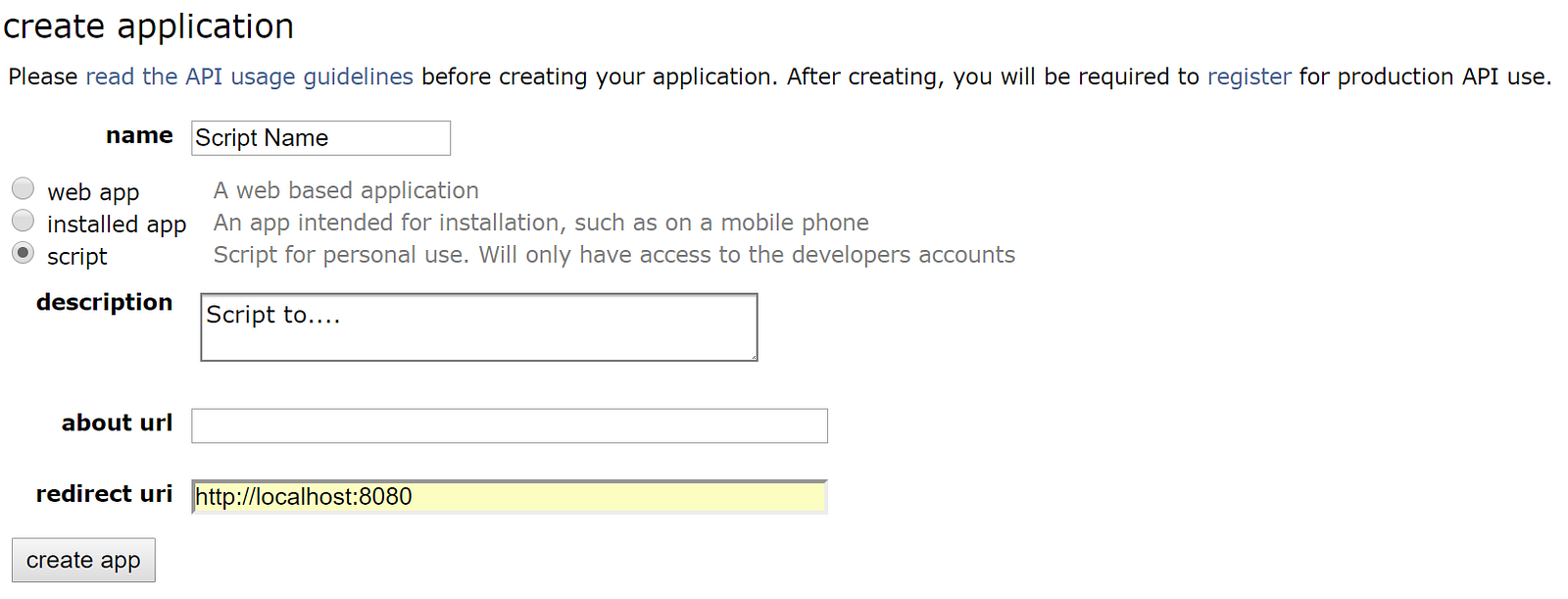
Hit the create app button once you have populated all fields. You should now have a script which resembles the following:

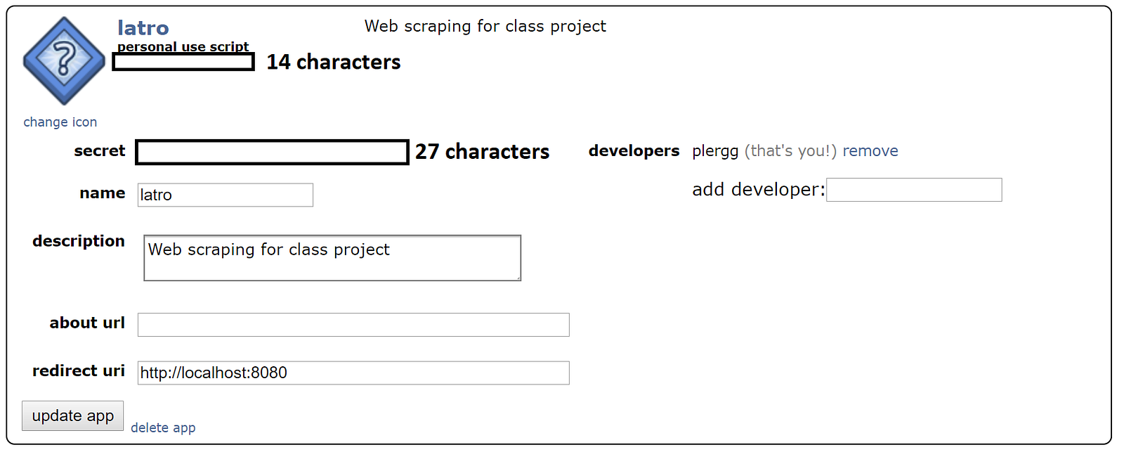
NOTE: Certain components of the reddit = praw.Reddit("BasyesianMethodsForHackers") code have been intentionally omitted. This is because praw requires a user ID for accessing Reddit. the praw function follows the following format:

reddit = praw.Reddit(client_id='PERSONAL_USE_SCRIPT_14_CHARS', \
                     client_secret='SECRET_KEY_27_CHARS ', \
                     user_agent='YOUR_APP_NAME', \
                     username='YOUR_REDDIT_USER_NAME', \
                     password='YOUR_REDDIT_LOGIN_PASSWORD')

For help with creating a Reddit instance, visit https://praw.readthedocs.io/en/latest/code_overview/reddit_instance.html.

For help on configuring PRAW, visit https://praw.readthedocs.io/en/latest/getting_started/configuration.html.

In [9]:

#@title Reddit API setup
import sys
import numpy as np
from IPython.core.display import Image
import praw

reset_sess()

enter_client_id = 'ZhGqHeR1zTM9fg'                  #@param {type:"string"}
enter_client_secret = 'keZdvIa1Ge257NKEm3v-eGEdv8M' #@param {type:"string"}
enter_user_agent = "bayesian_app"                   #@param {type:"string"}
enter_username = "ThisIsJustADemo"                  #@param {type:"string"}
enter_password = "EnterYourOwnInfoHere"             #@param {type:"string"}

subreddit_name = "showerthoughts"     #@param ["showerthoughts", "todayilearned", "worldnews", "science", "lifeprotips", "nottheonion"] {allow-input: true}

reddit = praw.Reddit(client_id=enter_client_id,
                     client_secret=enter_client_secret,
                     user_agent=enter_user_agent,
                     username=enter_username,
                     password=enter_password)
subreddit  = reddit.subreddit(subreddit_name)

# go by timespan - 'hour', 'day', 'week', 'month', 'year', 'all'
# might need to go longer than an hour to get entries...

timespan = 'day' #@param ['hour', 'day', 'week', 'month', 'year', 'all']

top_submissions = subreddit.top(timespan)

#adding a number to the inside of int() call will get the ith top post.
ith_top_post = 2   #@param {type:"number"}
n_sub = int(ith_top_post)

i = 0
while i < n_sub:
    top_submission = next(top_submissions)
    i += 1

top_post = top_submission.title

upvotes = []
downvotes = []
contents = []

for sub in top_submissions:
    try:
        ratio = sub.upvote_ratio
        ups = int(round((ratio*sub.score)/(2*ratio - 1))
                  if ratio != 0.5 else round(sub.score/2))
        upvotes.append(ups)
        downvotes.append(ups - sub.score)
        contents.append(sub.title)
    except Exception as e:
        continue

votes = np.array( [ upvotes, downvotes] ).T

print("Post contents: \n")
print(top_post)

Post contents: 

If giraffes were stealthy meat-eating predators with a taste for human flesh, they would stalk apartment complexes at night and wait for people to walk by their open windows.

Above is the top post as well as some other sample posts:

In [10]:

"""
contents: an array of the text from the last 100 top submissions to a subreddit
votes: a 2d numpy array of upvotes, downvotes for each submission.
"""
n_submissions_ = len(votes)
submissions = tfd.Uniform(low=float(0.), high=float(n_submissions_)).sample(sample_shape=(4))
submissions_ = evaluate(tf.cast(submissions,tf.int32))

print("Some Submissions (out of %d total) \n-----------"%n_submissions_)
for i in submissions_:
    print('"' + contents[i] + '"')
    print("upvotes/downvotes: ",votes[i,:], "\n")

Some Submissions (out of 98 total) 
-----------
"You are free to commit crime but you just have to face the consequences."
upvotes/downvotes:  [45  6] 

"You can burn yourself with water."
upvotes/downvotes:  [612  53] 

"Telling someone that she was made for you goes from romantic to selfish the more you think about it."
upvotes/downvotes:  [335  10] 

"Just need to flip the Flat Earth over so we can chill on the cool side for awhile"
upvotes/downvotes:  [162  20] 

For a given true upvote ratio $p$ and $N$ votes, the number of upvotes will look like a Binomial random variable with parameters $p$ and $N$ . (This is because of the equivalence between upvote ratio and probability of upvoting versus downvoting, out of $N$ possible votes/trials). We create a function that performs Bayesian inference on $p$ , for a particular submission's upvote/downvote pair.

In [0]:

def joint_log_prob(upvotes, N, test_upvote_ratio):
    """
    Args:
      upvotes: observed upvotes for a submission
      N : observed upvotes+downvotes for the submission
      test_upvote_ratio: hypothesized value for true value of upvote ratio
    Returns: 
      Joint log probability optimization function to compute true upvote ratio.
    """
    tfd = tfp.distributions

    # use a uniform prior
    rv_upvote_ratio = tfd.Uniform(name="upvote_ratio", low=0., high=1.)
    rv_observations = tfd.Binomial(name="obs",
                                   total_count=float(N),
                                   probs=test_upvote_ratio)
    return (
        rv_upvote_ratio.log_prob(test_upvote_ratio)
        + rv_observations.log_prob(float(upvotes))
    )

in some cases we might want to run someting like an HMC for multiple, or a variable number, of inputs. Loops are common examples of this. Here we define our function for setting up an HMC that can take in different numbers of upvotes and/or downvotes.

In [0]:

def posterior_upvote_ratio(upvotes, downvotes):
    reset_sess()
    
    burnin = 5000
    N = float(upvotes) + float(downvotes)

    # Initialize the step_size. (It will be automatically adapted.)
    with tf.variable_scope(tf.get_variable_scope(), reuse=tf.AUTO_REUSE):
        step_size = tf.get_variable(
          name='step_size',
          initializer=tf.constant(0.5, dtype=tf.float32),
          trainable=False,
          use_resource=True
        ) 

    # Set the chain's start state.
    initial_chain_state = [
        0.5 * tf.ones([], dtype=tf.float32, name="init_upvote_ratio")
    ]

    # Since HMC operates over unconstrained space, we need to transform the
    # samples so they live in real-space.
    unconstraining_bijectors = [
        tfp.bijectors.Sigmoid()          
    ]

    # Define a closure over our joint_log_prob.
    unnormalized_posterior_log_prob = lambda *args: joint_log_prob(upvotes, N, *args)

    hmc=tfp.mcmc.TransformedTransitionKernel(
        inner_kernel=tfp.mcmc.HamiltonianMonteCarlo(
            target_log_prob_fn=unnormalized_posterior_log_prob,
            num_leapfrog_steps=2,
            step_size=step_size,
            state_gradients_are_stopped=True),
        bijector=unconstraining_bijectors)

    hmc = tfp.mcmc.SimpleStepSizeAdaptation(
      inner_kernel=hmc, num_adaptation_steps=int(burnin * 0.8)
    )

    # Sample from the chain.
    [
        posterior_upvote_ratio
    ], kernel_results = tfp.mcmc.sample_chain(
        num_results=20000,
        num_burnin_steps=burnin,
        current_state=initial_chain_state,
        kernel=hmc)

    # Initialize any created variables.
    init_g = tf.global_variables_initializer()
    init_l = tf.local_variables_initializer()
    
    evaluate(init_g)
    evaluate(init_l)
    
    return evaluate([
        posterior_upvote_ratio,
        kernel_results,
    ])

In [13]:

plt.figure(figsize(11., 8))
posteriors = []
colours = ["#5DA5DA", "#F15854", "#B276B2", "#60BD68", "#F17CB0"]
for i in range(len(submissions_)):
    j = submissions_[i]
    posteriors.append( posterior_upvote_ratio(votes[j, 0], votes[j, 1])[0] )
    plt.hist( posteriors[i], bins = 10, normed = True, alpha = .9, 
            histtype="step",color = colours[i], lw = 3,
            label = '(%d up:%d down)\n%s...'%(votes[j, 0], votes[j,1], contents[j][:50]) )
    plt.hist( posteriors[i], bins = 10, normed = True, alpha = .2, 
            histtype="stepfilled",color = colours[i], lw = 3, )
    
plt.legend(loc="upper left")
plt.xlim( 0, 1)
plt.title("Posterior distributions of upvote ratios on different submissions");

WARNING:tensorflow:From /usr/local/lib/python3.6/dist-packages/tensorflow_probability/python/distributions/uniform.py:182: add_dispatch_support.<locals>.wrapper (from tensorflow.python.ops.array_ops) is deprecated and will be removed in a future version.
Instructions for updating:
Use tf.where in 2.0, which has the same broadcast rule as np.where

Some distributions are very tight, others have very long tails (relatively speaking), expressing our uncertainty with what the true upvote ratio might be.

Sorting!

We have been ignoring the goal of this exercise: how do we sort the submissions from best to worst? Of course, we cannot sort distributions, we must sort scalar numbers. There are many ways to distill a distribution down to a scalar: expressing the distribution through its expected value, or mean, is one way. Choosing the mean is a bad choice though. This is because the mean does not take into account the uncertainty of distributions.

I suggest using the 95% least plausible value, defined as the value such that there is only a 5% chance the true parameter is lower (think of the lower bound on the 95% credible region). Below are the posterior distributions with the 95% least-plausible value plotted:

In [14]:

N = posteriors[0].shape[0]
lower_limits = []
for i in range(len(submissions_)):
    j = submissions_[i]
    plt.hist( posteriors[i], bins = 20, normed = True, alpha = .9, 
            histtype="step",color = colours[i], lw = 3,
            label = '(%d up:%d down)\n%s...'%(votes[j, 0], votes[j,1], contents[j][:50]) )
    plt.hist( posteriors[i], bins = 20, normed = True, alpha = .2, 
            histtype="stepfilled",color = colours[i], lw = 3, )
    v = np.sort( posteriors[i] )[ int(0.05*N) ]
    plt.vlines( v, 0, 30 , color = colours[i], linestyles = "--",  linewidths=3  )
    lower_limits.append(v)
    plt.legend(loc="upper left")

plt.legend(loc="upper left")
plt.title("Posterior distributions of upvote ratios on different submissions");
order = np.argsort( -np.array( lower_limits ) )
print(order, lower_limits)

[2 1 3 0] [0.7836006, 0.9008505, 0.9514801, 0.8460546]

The best submissions, according to our procedure, are the submissions that are most-likely to score a high percentage of upvotes. Visually those are the submissions with the 95% least plausible value close to 1.

Why is sorting based on this quantity a good idea? By ordering by the 95% least plausible value, we are being the most conservative with what we think is best. When using the lower-bound of the 95% credible interval, we believe with high certainty that the 'true upvote ratio' is at the very least equal to this value (or greater), thereby ensuring that the best submissions are still on top. Under this ordering, we impose the following very natural properties:

given two submissions with the same observed upvote ratio, we will assign the submission with more votes as better (since we are more confident it has a higher ratio).
given two submissions with the same number of votes, we still assign the submission with more upvotes as better.

But this is too slow for real-time!

I agree, computing the posterior of every submission takes a long time, and by the time you have computed it, likely the data has changed. I delay the mathematics to the appendix, but I suggest using the following formula to compute the lower bound very fast.

\frac{a}{a + b} - 1.65\sqrt{ \frac{ab}{ (a+b)^2(a + b +1 ) } }

where $\begin{align} & a = 1 + u \\ & b = 1 + d \\ \end{align}$ $u$ is the number of upvotes, and $d$ is the number of downvotes. The formula is a shortcut in Bayesian inference, which will be further explained in Chapter 6 when we discuss priors in more detail.

In [15]:

def intervals(u, d):
    a = tf.add(1., u)
    b = tf.add(1., d)
    mu = tf.divide(x=a, y=tf.add(1., u))
    std_err = 1.65 * tf.sqrt((a * b) / ((a + b) ** 2 * (a + b + 1.)))
    
    return (mu, std_err)
  
print("Approximate lower bounds:")
posterior_mean, std_err  = evaluate(intervals(votes[:,0],votes[:,1]))
lb = posterior_mean - std_err
print(lb)
print("\n")
print("Top 40 Sorted according to approximate lower bounds:")
print("\n")
[ order ] = evaluate([tf.nn.top_k(lb, k=lb.shape[0], sorted=True)])
ordered_contents = []
for i, N in enumerate(order.values[:40]):
    ordered_contents.append( contents[i] )
    print(votes[i,0], votes[i,1], contents[i])
    print("-------------")

Approximate lower bounds:
[0.99269927 0.99397486 0.9954533  0.99409133 0.99016213 0.9921388
 0.9932303  0.9950698  0.9924482  0.9905308  0.99219704 0.9883038
 0.98586273 0.98920876 0.98701847 0.9825861  0.9784089  0.98187244
 0.9896374  0.98088    0.9845036  0.9757879  0.98391163 0.97651654
 0.9760173  0.96944773 0.97180194 0.98139995 0.984723   0.98333776
 0.97501504 0.98007494 0.9776715  0.9744575  0.97023726 0.9856403
 0.97080845 0.97544485 0.9791857  0.961427   0.9745684  0.9577916
 0.9674608  0.97471726 0.9576553  0.96101296 0.9536104  0.9696114
 0.9635106  0.9534545  0.95889676 0.9733387  0.9485553  0.95074564
 0.9599505  0.9509203  0.9458036  0.95018905 0.9485553  0.9536757
 0.94073695 0.95903665 0.95053595 0.9481962  0.96678776 0.9522802
 0.96910393 0.95128834 0.94423944 0.9413886  0.9619237  0.9421574
 0.94563764 0.9444311  0.9643911  0.94299465 0.9511917  0.9458798
 0.95053595 0.9304495  0.93613225 0.93222207 0.94465697 0.93661344
 0.9331166  0.94067496 0.9303111  0.9245648  0.9280292  0.938496
 0.92397803 0.93731874 0.9207582  0.9331846  0.9306861  0.9498649
 0.9209626  0.9306861 ]


Top 40 Sorted according to approximate lower bounds:


4750 648 Dragons would probably fear us as we can create water in our mouth
-------------
3983 254 Having a car the same age as you is lame. Having a car the same age as your parents is awesome.
-------------
3747 116 All pebbles seem small and insignificant until you get one get inside your shoes
-------------
2898 121 If you listen to slightly older music, you are out of the loop. But if you listen to really old music, you are listening to the classics.
-------------
2102 208 If everyone smelt bad no one would smell bad
-------------
2007 106 At some point in your life, you've probably made eye contact with a murderer, without even knowing it.
-------------
2208 92 The reason ghosts always make lights flash is because they are amazed by modern technology so just keep pressing the switch like a child.
-------------
2199 45 Most kids today will never have to face the awkwardness of calling a girl at home and having her dad answer the phone.
-------------
1777 74 If we could view life in the third person, we would probably spend a lot less time on our phones and watching TV because we would actually see ourselves mindlessly watching and/or scrolling.
-------------
893 28 The gasses found in Jupiter's atmosphere (ammonia, methane, etc) can cause brain damage, so those who go to Jupiter do, indeed, get more stupider.
-------------
914 19 Humans are probably the most consistently noisy animal to most other animals.
-------------
748 31 You'll never be in the same place in the universe ever again
-------------
727 46 If public libraries didn’t already exist, they’d be thought of now as the most impractical and unrealistic idea ever.
-------------
697 22 We tend to think that the knowledge we have today will be preserved forever. But actually the way we store information today is way less secure than ancient stone carvings.
-------------
618 26 A minor disadvantage to being older is that you have to scroll down further to select your birth year.
-------------
612 53 You can burn yourself with water.
-------------
544 74 We just walk around pretending it's not weird that one of our hands is better at stuff than the other.
-------------
513 39 "Pull Up" still reads as pull up backwards.
-------------
510 10 If you’re a short person, people are always looking down on you at a flattering selfie angle.
-------------
354 19 "Space" button on keyboard takes a lot of space for just a " ".
-------------
335 10 Telling someone that she was made for you goes from romantic to selfish the more you think about it.
-------------
321 28 A male mermaid would probably be a merbutler not a merman
-------------
322 10 If hydras were real, we’d probably farm them by hacking off their heads for an infinite food source
-------------
306 23 "Nice guys finish last" takes on a whole new meaning in a bedroom setting.
-------------
387 43 “You a real one” and “You are alone” is the same sentence, just with differently placed spaces
-------------
330 63 With self-driving Cars on the horizon, we’ll see some people suddenly die while in the car for any particular reason, and just arrive at their destination dead.
-------------
261 26 For adults, Halloween is a candy tax day in which children come around like irs agents to collect what you owe.
-------------
251 8 The dinosaur game is the only browser game where when your internet is better it gets laggier.
-------------
254 5 Empathy is a great emotion to have, but it can make you feel horrible
-------------
232 5 Some of the most beautiful singing voices will never be heard because the singers are too self conscious.
-------------
209 11 Songs that you like immediately usually don't last long, but songs that take a while to like usually last a long time.
-------------
207 6 We are all side characters in other people’s lives.
-------------
217 9 The reason a ghost will try to kill you is because it needs a friend.
-------------
204 11 We'll soon see gamers passing away of old age before being able to play the next installment of their favorite game franchise.
-------------
211 18 Once the internet disappears and all the books printed on acid-based paper the past 100 years decay, nothing will be left of our civilization except the highway system, skyscrapers, and billions of discarded water bottles.
-------------
193 2 Every house has an odor and it is kind of like the house’s personality.
-------------
162 9 People who are sensitive to smells could just say that they’re scentsitive
-------------
154 5 Every time you recall a memory you spend a portion of your current life reliving the life you already lived.
-------------
151 3 The worse you are the easier it is to improve.
-------------
162 20 Just need to flip the Flat Earth over so we can chill on the cool side for awhile
-------------

We can view the ordering visually by plotting the posterior mean and bounds, and sorting by the lower bound. In the plot below, notice that the left error-bar is sorted (as we suggested this is the best way to determine an ordering), so the means, indicated by dots, do not follow any strong pattern.

In [16]:

r_order = order.indices[::-1][-40:]
ratio_range_ = evaluate(tf.range( len(r_order)-1,-1,-1 )) 
r_order_vals = order.values[::-1][-40:]
plt.errorbar( r_order_vals, 
                             np.arange( len(r_order) ), 
               xerr=std_err[r_order], capsize=0, fmt="o",
                color = TFColor[0])
plt.xlim( 0.3, 1)
plt.yticks( ratio_range_ , map( lambda x: x[:30].replace("\n",""), ordered_contents) );

In the graphic above, you can see why sorting by mean would be sub-optimal.

Extension to Starred rating systems

The above procedure works well for upvote-downvotes schemes, but what about systems that use star ratings, e.g. 5 star rating systems. Similar problems apply with simply taking the average: an item with two perfect ratings would beat an item with thousands of perfect ratings, but a single sub-perfect rating.

We can consider the upvote-downvote problem above as binary: 0 is a downvote, 1 if an upvote. A $N$ -star rating system can be seen as a more continuous version of above, and we can set $n$ stars rewarded is equivalent to rewarding $\frac{n}{N}$ . For example, in a 5-star system, a 2 star rating corresponds to 0.4. A perfect rating is a 1. We can use the same formula as before, but with $a,b$ defined differently:

\frac{a}{a + b} - 1.65\sqrt{ \frac{ab}{ (a+b)^2(a + b +1 ) } }

where $\begin{align} & a = 1 + S \\ & b = 1 + N - S \\ \end{align}$ where $N$ is the number of users who rated, and $S$ is the sum of all the ratings, under the equivalence scheme mentioned above.

Example: Counting Github stars

What is the average number of stars a Github repository has? How would you calculate this? There are over 6 million respositories, so there is more than enough data to invoke the Law of Large numbers. Let's start pulling some data.

In [17]:

reset_sess()

import wget
url = 'https://raw.githubusercontent.com/CamDavidsonPilon/Probabilistic-Programming-and-Bayesian-Methods-for-Hackers/master/Chapter3_MCMC/data/github_data.csv'
filename = wget.download(url)
filename

'github_data.csv'

In [18]:

# Github data scrapper
# See documentation_url: https://developer.github.com/v3/

from json import loads
import datetime
import numpy as np
from requests import get

"""
variables of interest:
    indp. variables
    - language, given as a binary variable. Need 4 positions for 5 langagues
    - #number of days created ago, 1 position
    - has wiki? Boolean, 1 position
    - followers, 1 position
    - following, 1 position
    - constant
    
    dep. variables
    -stars/watchers
    -forks
"""


MAX = 8000000
today =  datetime.datetime.today()
randint = np.random.randint
N = 20 #sample size. 
auth = ("mikeshwe", "kick#Ass1" )

language_mappings = {"Python": 0, "JavaScript": 1, "Ruby": 2, "Java":3, "Shell":4, "PHP":5}

#define data matrix: 
X = np.zeros( (N , 12), dtype = int )

for i in range(N):
    is_fork = True
    is_valid_language = False
    
    while is_fork == True or is_valid_language == False:
        is_fork = True
        is_valid_language = False
        
        params = {"since":randint(0, MAX ) }
        r = get("https://api.github.com/repositories", params = params, auth=auth )
        results = loads( r.text )[0]
        #im only interested in the first one, and if it is not a fork.
        #print(results)
        is_fork = results["fork"]
        
        r = get( results["url"], auth = auth)
        
        #check the language
        repo_results = loads( r.text )
        try: 
            language_mappings[ repo_results["language" ] ]
            is_valid_language = True
        except:
            pass

    #languages 
    X[ i, language_mappings[ repo_results["language" ] ] ] = 1
    
    #delta time
    X[ i, 6] = ( today - datetime.datetime.strptime( repo_results["created_at"][:10], "%Y-%m-%d" ) ).days
    
    #haswiki
    X[i, 7] = repo_results["has_wiki"]
    
    #get user information
    r = get( results["owner"]["url"] , auth = auth)
    user_results = loads( r.text )
    X[i, 8] = user_results["following"]
    X[i, 9] = user_results["followers"]
    
    #get dep. data
    X[i, 10] = repo_results["watchers_count"]
    X[i, 11] = repo_results["forks_count"]
    print()
    print(" -------------- ")
    print(i, ": ", results["full_name"], repo_results["language" ], repo_results["watchers_count"], repo_results["forks_count"]) 
    print(" -------------- ") 
    print() 
    
np.savetxt("github_data.csv", X, delimiter=",", fmt="%d" )

 -------------- 
0 :  josephj/f2e-class PHP 14 1
 -------------- 


 -------------- 
1 :  bellini666/gnome-shell-notifications-alert JavaScript 38 12
 -------------- 


 -------------- 
2 :  PanKleszcz/ET Java 1 0
 -------------- 


 -------------- 
3 :  Yorda/SolnRss Java 0 0
 -------------- 


 -------------- 
4 :  Jefersonandrade/Vendas Java 1 0
 -------------- 


 -------------- 
5 :  raduwen/HackathonGameDevelopWikiSamples Ruby 0 0
 -------------- 


 -------------- 
6 :  kdmny/redmine-heroku Ruby 47 7
 -------------- 


 -------------- 
7 :  stewartduffy/contact_form PHP 1 0
 -------------- 


 -------------- 
8 :  bluedynamics/bda.bfg.tile Python 1 1
 -------------- 


 -------------- 
9 :  eldog/fmobile Java 6 2
 -------------- 


 -------------- 
10 :  KimiyukiYamauchi/Memopad Java 0 0
 -------------- 


 -------------- 
11 :  sheldonh/life Ruby 1 0
 -------------- 


 -------------- 
12 :  Curacion/demo_app Ruby 1 0
 -------------- 


 -------------- 
13 :  sunaku/inochi Ruby 10 2
 -------------- 


 -------------- 
14 :  gokzz/twitter Ruby 1 0
 -------------- 


 -------------- 
15 :  ryanj/twitGrep JavaScript 3 0
 -------------- 


 -------------- 
16 :  xiaomen/selfstudy JavaScript 2 1
 -------------- 


 -------------- 
17 :  artem-bochkarev/PPMA_HOME_TASK Java 0 0
 -------------- 


 -------------- 
18 :  tc/tc.github.com JavaScript 0 0
 -------------- 


 -------------- 
19 :  olivopaolo/boing Python 3 0
 -------------- 

Conclusion

While the Law of Large Numbers is cool, it is only true so much as its name implies: with large sample sizes only. We have seen how our inference can be affected by not considering how the data is shaped.

By (cheaply) drawing many samples from the posterior distributions, we can ensure that the Law of Large Number applies as we approximate expected values (which we will do in the next chapter).
Bayesian inference understands that with small sample sizes, we can observe wild randomness. Our posterior distribution will reflect this by being more spread rather than tightly concentrated. Thus, our inference should be correctable.
There are major implications of not considering the sample size, and trying to sort objects that are unstable leads to pathological orderings. The method provided above solves this problem.

Appendix

Derivation of sorting submissions formula

Basically what we are doing is using a Beta prior (with parameters $a=1, b=1$ , which is a uniform distribution), and using a Binomial likelihood with observations $u, N = u+d$ . This means our posterior is a Beta distribution with parameters $a' = 1 + u, b' = 1 + (N - u) = 1+d$ . We then need to find the value, $x$ , such that 0.05 probability is less than $x$ . This is usually done by inverting the CDF (Cumulative Distribution Function), but the CDF of the beta, for integer parameters, is known but is a large sum [3].

We instead use a Normal approximation. The mean of the Beta is $\mu = a'/(a'+b')$ and the variance is

\sigma^2 = \frac{a'b'}{ (a' + b')^2(a'+b'+1) }

Hence we solve the following equation for $x$ and have an approximate lower bound.

0.05 = \Phi\left( \frac{(x - \mu)}{\sigma}\right)

$\Phi$ being the cumulative distribution for the normal distribution

Exercises

1. How would you estimate the quantity $E\left[ \cos{X} \right]$ , where $X \sim \text{Exp}(4)$ ? What about $E\left[ \cos{X} | X \lt 1\right]$ , i.e. the expected value given we know $X$ is less than 1? Would you need more samples than the original samples size to be equally accurate?

In [19]:

## Enter code here
%%time
import tensorflow as tf
import tensorflow_probability as tfp
tfd = tf.distributions

exp = tfd.Exponential(rate=4.)
N = 10000
X = exp.sample(sample_shape=int(N))
with tf.Session() as exercise_1:
  print(X.eval())
  
## ...

WARNING:tensorflow:From <timed exec>:5: Exponential.__init__ (from tensorflow.python.ops.distributions.exponential) is deprecated and will be removed after 2019-01-01.
Instructions for updating:
The TensorFlow Distributions library has moved to TensorFlow Probability (https://github.com/tensorflow/probability). You should update all references to use `tfp.distributions` instead of `tf.distributions`.
WARNING:tensorflow:From /usr/local/lib/python3.6/dist-packages/tensorflow/python/ops/distributions/exponential.py:114: Gamma.__init__ (from tensorflow.python.ops.distributions.gamma) is deprecated and will be removed after 2019-01-01.
Instructions for updating:
The TensorFlow Distributions library has moved to TensorFlow Probability (https://github.com/tensorflow/probability). You should update all references to use `tfp.distributions` instead of `tf.distributions`.
WARNING:tensorflow:From /usr/local/lib/python3.6/dist-packages/tensorflow/python/ops/distributions/gamma.py:181: Distribution.__init__ (from tensorflow.python.ops.distributions.distribution) is deprecated and will be removed after 2019-01-01.
Instructions for updating:
The TensorFlow Distributions library has moved to TensorFlow Probability (https://github.com/tensorflow/probability). You should update all references to use `tfp.distributions` instead of `tf.distributions`.
[0.4458776  0.30991256 0.13016596 ... 0.21326569 0.25109488 0.18059786]
CPU times: user 37.8 ms, sys: 3.66 ms, total: 41.5 ms
Wall time: 65.3 ms

2. The following table was located in the paper "Going for Three: Predicting the Likelihood of Field Goal Success with Logistic Regression" [2]. The table ranks football field-goal kickers by their percent of non-misses. What mistake have the researchers made?

Kicker Careers Ranked by Make Percentage

Rank	Kicker	Make %	Number of Kicks
1	Garrett Hartley	87.7	57
2	Matt Stover	86.8	335
3	Robbie Gould	86.2	224
4	Rob Bironas	86.1	223
5	Shayne Graham	85.4	254
…	…	…
51	Dave Rayner	72.2	90
52	Nick Novak	71.9	64
53	Tim Seder	71.0	62
54	Jose Cortez	70.7	75
55	Wade Richey	66.1	56

In August 2013, a popular post on the average income per programmer of different languages was trending. Here's the summary chart: (reproduced without permission, cause when you lie with stats, you gunna get the hammer). What do you notice about the extremes?

Average household income by programming language

Language	Average Household Income ($)	Data Points
Puppet	87,589.29	112
Haskell	89,973.82	191
PHP	94,031.19	978
CoffeeScript	94,890.80	435
VimL	94,967.11	532
Shell	96,930.54	979
Lua	96,930.69	101
Erlang	97,306.55	168
Clojure	97,500.00	269
Python	97,578.87	2314
JavaScript	97,598.75	3443
Emacs Lisp	97,774.65	355
C#	97,823.31	665
Ruby	98,238.74	3242
C++	99,147.93	845
CSS	99,881.40	527
Perl	100,295.45	990
C	100,766.51	2120
Go	101,158.01	231
Scala	101,460.91	243
ColdFusion	101,536.70	109
Objective-C	101,801.60	562
Groovy	102,650.86	116
Java	103,179.39	1402
XSLT	106,199.19	123
ActionScript	108,119.47	113

References

Wainer, Howard. The Most Dangerous Equation. American Scientist, Volume 95.
Clarck, Torin K., Aaron W. Johnson, and Alexander J. Stimpson. "Going for Three: Predicting the Likelihood of Field Goal Success with Logistic Regression." (2013): n. page. Web. 20 Feb. 2013.
http://en.wikipedia.org/wiki/Beta_function#Incomplete_beta_function