
# A function of 3 variables:
f(x,y,z) = (x^2 + y^2) * z

# Can evaluate the function at any point:
f(1,0,2)

# There are several ways to get partial derivatives:
f.diff(x)
f.derivative(x)
derivative(f,x)
derivative(f,z)
# Note that the answer is returned in function notation,
# with inputs to the left and outputs to the right of the arrow.

# It is easy to compute the gradient of f:
f.gradient()
2
(x, y, z) |--> 2*x*z
(x, y, z) |--> 2*x*z
(x, y, z) |--> 2*x*z
(x, y, z) |--> x^2 + y^2
(x, y, z) |--> (2*x*z, 2*y*z, x^2 + y^2)


# Step 0: Define the function:
g(x,y) = 100*(y - x^2)^2 + (1 - x)^2

# Step 1: Find the points where the gradient of g = 0:
gx(x,y) = derivative(g,x)        # Find derivative of g with respect to x.
gy(x,y) = derivative(g,y)        # Derivative of g with respect to y.
results = solve([gx == 0, gy ==0], (x,y), solution_dict=True)
    # Note that results[0] is a dictionary containing the solutions
xval = results[0][x]
yval = results[0][y]
print "Gradient is 0 at: x =", xval, "y =", yval

# Step 2: Check sign of gxx and determinant of Hessian matrix at those points:
gh = g.hessian()                  # Find the Hessian matrix (in function form)
gh(xval,yval).determinant()       # Compute its determinant at (1,1)
gxx(x,y) = derivative(gx,x)       # Find gxx as function of (x,y)
gxx(xval,yval)                    # Compute its value at (1,1)

# Step 3: Since the Hessian and gxx are both positive at (1,1), it is a local minimum.
# Answer: g(1,1)=0 is a local minimum of the given function g(x,y).
#         Since grad(g) != 0 anywhere else, there is no other
#         local minimum/maximum.
Gradient is 0 at: x = 1 y = 1
400
802

# It is important to keep the distinction between independent variable(s),
# and the vector components, clear in your own mind.

x = var('x')   # The single independent variable

# (1) A 3-component vector:
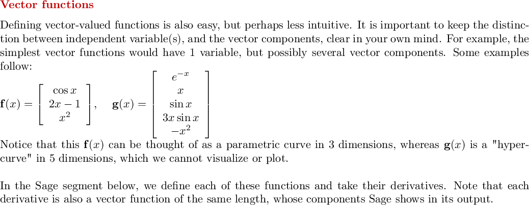
fv = vector( (cos(x), 2*x-1, x^2) )
fv(x=4)   # Evaluate fv at x=4. Note that fv(4) also currently works, but is to be discontinued soon.
derivative(fv, x)  # 1st derivative of fv (which is also a vector function).
parametric_plot(fv, (x,-2,3), thickness='3')  # Just to see what the function looks like.

# (2) A 5-component vector and its derivative:
gv = vector( (e^-x, x, sin(x), 3*x*sin(x), -x^2) )
derivative(gv, x)
(cos(4), 7, 16)
(-sin(x), 2, 2*x)
3D rendering not yet implemented
(-e^(-x), 1, cos(x), 3*x*cos(x) + 3*sin(x), -2*x)

# Here's how to define vector functions of multiple variables.
# Notice, it is an intuitive generalization of the previous syntax.
#
x, y, z = var('x, y, z')
f = vector( (x^2 + y^2, 3*x*y))
g = vector( (x^2 * y, x^2 * z, y*z) )

# You can evaluate the functions at any specific point by
# similarly generalizing the single variable syntax.
# (I've used the print command just to show the output clearly):
print "f(0,2)=",  f(x=0, y=2)
print "g(1,2,3)=", g(x=1, y=2, z=3)

# Find divergence and curl. Note, the syntax requires
# specifying the names of the variables in order.  (Again,
# the print command is just to show the output clearly):
print "div(f)=", f.div([x,y])
print "curl(f)=", f.curl([x,y])
print "div(g)=", g.div([x,y,z])
print "curl(g)=", g.curl([x,y,z])
f(0,2)= (4, 0)
g(1,2,3)= (2, 3, 6)
div(f)= 5*x
curl(f)= y
div(g)= 2*x*y + y
curl(g)= (-x^2 + z, 0, -x^2 + 2*x*z)

# It is easy to find partial derivatives. Note that each
# partial derivative is itself a vector function.
print "partial derivatives of f:"
derivative(f, x)  # partial of f with respect to x.
derivative(f, y)  # partial of f with respect to y.

print " "
print "partial derivatives of g:"
derivative(g, x)  # partial of g with respect to x.
derivative(g, y)  # partial of g with respect to y.
derivative(g, z)  # partial of g with respect to z.
partial derivatives of f:
(2*x, 3*y)
(2*y, 3*x)
partial derivatives of g:
(2*x*y, 2*x*z, 0)
(x^2, 0, z)
(0, x^2, y)

# Example to illustrate the meaning of partial derivatives in a 2-variable function.
# x-derivative gives tangent line parallel to x-direction;
# y-derivative gives tangent line parallel to y-direction.

x, y, t = var('x y t')
fs = sin(x) + cos(y)      # An example function
Q = plot3d(fs, (x,-3,3), (y,-3,3) )
fsx = derivative(fs,x)    # Derivative in x-direction
fsy = derivative(fs,y)    # Derivative in y-direction
xp = 1.5; yp = -1         # Some sample point in the domain of interest

# Tangent in x-direction in parametric form: (xp+t, yp, fsx*t+fs)
R = parametric_plot( (t+xp, yp, t*fsx(x=xp,y=yp)+fs(x=xp,y=yp)), (t,-3,3), thickness=3, color='green' )
# Tangent in y-direction in parametric form: (xp, yp+t, fsy*t+fs)
S = parametric_plot( (xp, t+yp, t*fsy(x=xp,y=yp)+fs(x=xp,y=yp)), (t,-3,3), thickness=3, color='yellow' )
T = point([xp,yp,fs(x=xp,y=yp)], size=10, color='black')
show(Q+R+S+T)
3D rendering not yet implemented

Interact: please open in CoCalc

# Tangent plane example.  Here the tangent plane at the point (c,d) has
# the parametric form: x = s+c, y = t+d, z = s*fx(c,d) + t*fy(c,d) + f(c,d)
# for $s, t \in (-\infty,\infty)$.

x, y, s, t = var('x y s t')
fs = sin(x) + cos(y)
Q = plot3d(fs, (x,-3,3), (y,-3,3) )
fsx = derivative(fs,x)    # Derivative in x-direction
fsy = derivative(fs,y)    # Derivative in y-direction
xp = 2; yp = -0.5         # Some sample point in the domain of interest
R = parametric_plot( (s+xp, t+yp, s*fsx(x=xp,y=yp)+t*fsy(x=xp,y=yp)+fs(x=xp,y=yp)), (t,-3,3), (s,-3,3), thickness=3, color='yellow', opacity=0.3 )
T = point([xp,yp,fs(x=xp,y=yp)], size=10, color='black')
show(Q+R+T)
3D rendering not yet implemented

x = var('x')
integral(x^2, x)          # Indefinite integral
integral(x^2, (x,0,1))    # Definite integral
1/3*x^3
1/3

x, y = var('x, y')
integral(integral(x^2*sin(y), y), x)               # Indefinite integral
integral(integral(x^2*sin(y), (y,0,pi)), (x,0,1))  # Definite integral
-1/3*x^3*cos(y)
2/3

# Formula for the area of a circle using double integration
x,y, r = var('x y r')
assume(r>0)               # This is needed to to prevent complaints from Sage!
integral(integral(1, (y,-sqrt(r^2-x^2),sqrt(r^2-x^2))), (x,-r,r))
pi*r^2