\( % theorem \newenvironment{pf}{\textbf{Proof.}}{\rule{1ex}{1ex}} \newtheorem{qu}{Question} \newtheorem{thm}{Theorem} \newtheorem{rmk}{Remark} \newtheorem{go}{Goal} \newtheorem{df}{Definition} \newtheorem{prop}{Proposition} \newtheorem{mot}{Motivation} \newtheorem{ex}{Example} \lstnewenvironment{code}{}{} \newcommand{\nc}{\newcommand} %% env \nc{\env}[2]{ \begin{#1} #2 \end{#1} } \nc{\arr}[2]{ \begin{array}{#1} #2 \end{array} } \nc{\arrb}[2]{ \left\{ \begin{array}{#1} #2 \end{array} \right. } \nc{FTC}[3]{ \left[#3\right]^{#2}_{#1} } \nc{\bracs}[1]{ \left[#1\right] } \nc{\brac}[1]{ \left(#1\right) } \nc{\bracp}[1]{ \left\{#1\right\} } \nc{\intd}[4]{\int^{#2}_{#1}\left(#3\right) #4} % shortcut \nc{\Lra}{\Leftrightarrow} \nc{\Ra}{\Rightarrow} \nc{\La}{\Leftarrow} \nc{\C}{\mathbb{C}} \nc{\R}{\mathbb{R}} \nc{\Fc}{\mathcal{C}} \nc{\bds}{\boldsymbol} \nc{\ds}{\displaystyle} % begin end \nc{\bit}{\begin{itemize}} \nc{\eit}{\end{itemize}} \nc{\bcode}{\begin{code}} \nc{\ecode}{\end{code}} \nc{\bsage}{\begin{sageblock}} \nc{\esage}{\end{sageblock}} %pic \nc{\pic}{\includegraphics} \nc{\svg}{\includesvg} \nc{\pica}{\includegraphics[width=100px,height=100px]} \nc{\picb}{\includegraphics[width=150px,height=150px]} \nc{\vs}{\vspace} \nc{\tbf}{\textbf} %arrow \nc{\upa}{\nearrow} \nc{\downa}{\searrow} \nc{\upw}{\rcurvearrowright} \nc{\downw}{\curvearrowright} \)

MA441- LEC 1

Goal

  • Understanding the movitation of calculus
  • Understanding the tangent line of a curve.
  • average and instantaneous velocity

Two strategies in mathematics/computer science

Divide and conquer

  • Break the problem into sub-problems
  • Solve the trivial cases
  • Combine sub-problems to the original problem.

Reduction Method

Assume problem A is reducible to an easy problem B. If we can solve problem B, then we can solve problem A.

Why Calculus?

  • Area problem
  • Tangent line

Area problem I

Approximating Area of a Circle

Area problem II

Approximating area of a function

tangent line

"Tangent" means touching. So tangent line to a curve is a line that touches the curve.

The Secant line \(\overline{PQ}\) is the line passing through point \(P\) and \(Q\).

How can you find the slope of the secant line \(\overline{PQ}\), \(m_{PQ}\)?

Tangent and secant

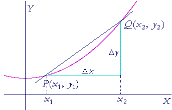
\[m_{PQ}=\frac{y_2-y_1}{x_2-x_1}\]

How can you calculate the slope of tangent line at a point \(P\)?

Find the slope of tangent line of \(f(x)=\frac{x^2}{4}\) at \(x=2\).

From above experiment, what do you expect?

Physics

Let \(y=f(x)\) be a position function of a car at time \(x\).


\[ average~velocity=\frac{\Delta distance}{\Delta time}=\frac{\Delta y}{\Delta x} \]

which is the slope of secant line.

How about an instantaneous velocity at time \(x\)?


\[ instantaneous~velocity =?=slope~of~tangent~line \]

History

Newton

newton

Born: 25 December 1642

Principia Mathematica(1687)

Principia Mathematica

Wiki

Calculus