################################
#
#     TABLE OF CONTENTS
#     (You can move to any line by using the "lightning bolt" button to the right of the large 'A')
#
#  60  3D grapher
# 160  Vectors and Points
# 208  planes and angles of tetrahedron
# 228  Two defined functions for drawing axes and planes. Useful for inserting into your pictures
# 272  Computation of curvature, etc.
# 395  Solution to 13.2.28
# 453  Interactive 3D grapher.  Very useful!
# 555  Parametric curve and osculating plane (includes graphs of curvature, velocity, acceleration)
# 704  Interactive TANGENT PLANE PLOTTER.  Very useful!  Includes partial derivatives!
# 802  plot compared with contour plot
# 827  Chain-rule practice: great homework helper allows you to define complicated functions and find partial derivatives
# 870  Definite integrals, included iterated multiple integrals
# 885  Some simple code to empirically play with probability distributions
# 930  Interactive change-of-variables and Jacobian explorer
# 969  PLOTTING VECTOR FIELDS. Simple example with gradient field and level curves.
##########################################################
#
#
#  3D grapher
#
#
##########################################################

# There are several ways to define and plot 3-d functions.  The simplest is the z=f(x,y) form.
# For example, z = x^2+y^2.

# You can also define a function implicitly.  This is sometimes more illuminating. For example, a sphere is
# more easily defined as the solution set to x^2+y^2+z^2=r^2 for some constant r.  In this example, we will use some of each.

# define variables (usually x is understood to be a symbolic variable, but define it just in case)
%var x,y,z

###############################################################################################
#define function(s).  This code includes an optional second function; you can put in as many as you want
f1 = x^2-y^2  #we will plot this with the plot_3d command, the z=f(x,y) method
f2 = x-y^2+z^2    #we will plot this (plane) with the implicit_plot3d command, using f(x,y,z)=constant method.
f3 = x #This will be a
#
# IMPORTANT POINT ABOUT IMPLICIT PLOT: The default will plot f(x,y,z)=0, but if you want, you can pick a different value instead of 0, or
# for simplicity, just write the function so that it is in that form.  In other words, a sphere will use the function
# f(x,y,z) = x^2+y^2+z^2-r^2.
# If you prefer to use f(x,y,z)=constant, you can use the option "contour".  For example, these two lines both produce a sphere centered
# at the origin with radius 10
# implict_plot3d(x^2+y^2+z^2-100, (x,-10,10), (y,-10,10), (z,-10,10))
# implict_plot3d(x^2+y^2+z^2, (x,-10,10), (y,-10,10), (z,-10,10), contour = 100)
#
##############################################################################################

#define x, y, z limits
t=3
xvals=(x,-t,t); yvals = (y,-t,t)
zvals = (z,-t,t) #note that we don't need zvals except for implicitly defined functions.
#NOTE THAT THESE VALUES WILL NOT DISPLAY ALL OF THE SPHERE (f3)

#########################################################################
#AXES
origin=(0,0,0)
#set size (for how long axes are). This is a bit larger than the
#max of the largest x, y val; you may want to change it based on your function
size = 1.1*max(xvals[2],yvals[2],zvals[2])
xSize=size; ySize= size; zSize=size
xAxis = plot(vector((xSize,0,0)),color='blue',width=3)
yAxis = plot(vector((0,ySize,0)),color='red',width=3)
zAxis = arrow3d(origin,(0,0,zSize),color='green',width=3)
#Labels for axes
#set fontsize (change if you need to)
fsize=20
xT=text3d("X",(xSize*1.1,0,0),color='blue',fontsize=fsize)
yT=text3d("Y",(0,ySize*1.1,0),color='red',fontsize=fsize)
zT=text3d("Z",(0,0,zSize*1.1),color='green',fontsize=fsize)
axes = xAxis+xT+yAxis+yT+zAxis+zT
################################################################################

#OPTIONS
#first, options for each function.  these are numbered since there may be more than one.

# mesh? Usually we want it (1, otherwise 0)
mval1 = 1
mval2 = 0
mval3 = 0
#color
clr1='green'
clr2='green'
clr3='blue'

#opacity
opval1=1.0 #completely opaque
opval2=0.3 #more transparent
opval3=0.2

################################################################################

# Now, options for the entire thing

#frame?
frameval=true
#aspect ratio. Use simply 1 for true scale, sometimes we don't want true scale, in which case we use three values for x,y,z.
asp = [1,1,1]
#spin? (0 for no spin, positive numbers for faster)
spinval = 5

# Now, we create our function plots
#Define P1, P2 to be the plot of our function

P1=plot3d(f1,xvals,yvals, mesh=mval1, color=clr1,opacity=opval1)
P2=implicit_plot3d(f2,xvals,yvals,zvals, mesh=mval2, color=clr2,opacity=opval2)
P3=implicit_plot3d(f3,xvals,yvals,zvals, mesh=mval3, color=clr3,opacity=opval3)

#now we display P1, P2 and the axes.  If you don't want the axes, leave them out.
show(P2+P3+axes, frame=frameval, aspect_ratio=asp, spin=spinval)
3D rendering not yet implemented
############################################
#
# VECTORS AND POINTS
#
###############################################
#
# We used both points and vectors in the the construction of axes in the plots above.  The main idea is that points are indicated
# by ordered triples (x,y,z) with parentheses, and VECTORS are created using the 'vector' function; its input is a tuple.
# Thus, if P=(x,y,z) is a point, then vector(P) is a vector.  When you plot it, you get an arrow!

#
# First, let's define axes to put in our picture.  I'm just copying from above and adapting slightly. This code actually uses vectors for
             # the x and y axes, and just for variety, uses another construction for the z-axis.

#AXES
origin=(0,0,0)
#set size (for how long axes are).
size = 10
xSize=size; ySize= size; zSize=size

xAxis = plot(vector((xSize,0,0)),color='blue',width=3)
yAxis = plot(vector((0,ySize,0)),color='red',width=3)
zAxis = arrow3d(origin,(0,0,zSize),color='green',width=3)
#Labels for axes
#set fontsize (change if you need to)
fsize=20
xT=text3d("X",(xSize*1.1,0,0),color='blue',fontsize=fsize)
yT=text3d("Y",(0,ySize*1.1,0),color='red',fontsize=fsize)
zT=text3d("Z",(0,0,zSize*1.1),color='green',fontsize=fsize)

#AXES DEFINED here
axes = xAxis+xT+yAxis+yT+zAxis+zT
################################################################################

# Now let's define a few points and vectors, do some computations, and display them
a = (1,1,1)
pa = point(a, color='red',size=20,opacity=0.4)
b = (2,3,-1)
vb = plot(vector(b), color='green', width=4)

show(vb+axes+pa)
3D rendering not yet implemented
X=vector((1,2,3)); Y= vector((-1,3,5))
X.dot_product(Y)
X.cross_product(Y)
norm(X)
20
(1, -8, 5)
sqrt(14)
#planes and angles of a tetrahedron
a=(0,0,0); b= (0,1,1); c= (1,0,1); d= (1,1,0)
A = vector(a); B=vector(b); C=vector(c); D= vector(d)
# for plane BCD, compute vectors
CB = B-C
CD = D-C
N1 = CB.cross_product(CD)  #normal to plane
#now plane ACD
AC = C-A
AD = D-A
N2= AC.cross_product(AD)

#find angle between N1,2
N1.dot_product(N2)/(norm(N1)*norm(N2))
-1/3
n(acos(-1/3)*180/pi) #the n command converts to numerical form
109.471220634491
####################################################################
#
# Two defined functions for drawing axes and planes. Useful for inserting into your pictures
#
################################################################
def axes(size,xcolor='red',ycolor='green',zcolor='blue'):
    #returns a plot of axis vectors, labeled, with length equal to the 'size' argument
    #Note the OPTIONAL color arguments.  If you leave them out, the xyz axes are red, green, blue, respectively
    #But, for example, the command axes(12,xcolor='black') would produce axes of length 12 with x in black and the others
    #still in green and blue.

    xSize=size; ySize= size; zSize=size
    xAxis = plot(vector((xSize,0,0)),color=xcolor,width=3)
    yAxis = plot(vector((0,ySize,0)),color=ycolor,width=3)
    zAxis = plot(vector((0,0,zSize)),color=zcolor,width=3)
    #Labels for axes
    #set fontsize (change if you need to)
    fsize=20
    xT=text3d("X",(xSize*1.1,0,0),color=xcolor,fontsize=fsize)
    yT=text3d("Y",(0,ySize*1.1,0),color=ycolor,fontsize=fsize)
    zT=text3d("Z",(0,0,zSize*1.1),color=zcolor,fontsize=fsize)
    return xAxis+xT+yAxis+yT+zAxis+zT
###############################################################################

def plotPlane(N,P,s,clr='grey',op=0.2,meshvalue=0,show_normal=False):
    x,y,z=var('x y z')
    #N=normal vec, P = point (vector), s=size
    #This returns a plot of plane with the given normal vector and point, with x,y,z going plus or minus s units from the point.
    #optional arguments for color and opacity (default is nearly transparent grey)
    #the show_normal argument, if set to "true," will draw the normal vector N starting from the point P
    output = implicit_plot3d(N.dot_product(vector((x,y,z)))-N.dot_product(P),(x,P[0]-s,P[0]+s),(y,P[1]-s,P[1]+s),(z,P[2]-s,P[2]+s),color=clr,opacity=op,mesh=meshvalue)
    if show_normal:
        output += plot(N, start =P, color='black')
    #output += plot(N, start =P, color='black')
    return output

#Here are examples of using these
# Start with a variable to hold the plot objects.
P = axes(12)  #so P is the plot object.  We will increment with other stuff

P += plotPlane(vector((1,1,1)),vector((2,-1,5)),5,'yellow')
P += plotPlane(vector((0,0,1)),vector((0,0,4)),5,'blue', show_normal=True)

show(P, spin=5)
3D rendering not yet implemented
# Computation of curvature, etc.
%var t
x(t) = t; y(t) = t^2; z(t) = t^3

r(t) = (x(t),y(t),z(t))
v=r.diff(t) #velocity! The "diff" suffix does symbolic differentiation
a=r.diff(t,2)    #acceleration (the "2" means second derivative)

#Our convention is to use upper-case for vectors
R = vector(r); V= vector(v); A = vector(a)

#Now compute unit tangent and unit normal vectors.
#recall that norm() computes magnitude of a vector
T = V/norm(V) #unit tangent vector (function of t)
Tprime = T.diff(t) #derivative of unit tangent
#turn this into a unit normal
N = Tprime/norm(Tprime)

#curvature (two ways; should be equal)
K1 = norm(Tprime)/norm(V)
K2 = norm(V.cross_product(A))/(norm(V))^3
##########################################################
#
#
#  3D grapher
#
#
##########################################################

# There are several ways to define and plot 3-d functions.  The simplest is the z=f(x,y) form.
# For example, z = x^2+y^2.

# You can also define a function implicitly.  This is sometimes more illuminating. For example, a sphere is
# more easily defined as the solution set to x^2+y^2+z^2=r^2 for some constant r.  In this example, we will use some of each.

# define variables (usually x is understood to be a symbolic variable, but define it just in case)
%var x,y,z

###############################################################################################
#define function(s).  This code includes an optional second function; you can put in as many as you want
f1 = x^2-y^2  #we will plot this with the plot_3d command, the z=f(x,y) method
f2 = x^2+y^2+4*z^2-4    #we will plot this (plane) with the implicit_plot3d command, using f(x,y,z)=constant method.
f3 = x^2+y^2-1 #This will be a
#
# IMPORTANT POINT ABOUT IMPLICIT PLOT: The default will plot f(x,y,z)=0, but if you want, you can pick a different value instead of 0, or
# for simplicity, just write the function so that it is in that form.  In other words, a sphere will use the function
# f(x,y,z) = x^2+y^2+z^2-r^2.
# If you prefer to use f(x,y,z)=constant, you can use the option "contour".  For example, these two lines both produce a sphere centered
# at the origin with radius 10
# implict_plot3d(x^2+y^2+z^2-100, (x,-10,10), (y,-10,10), (z,-10,10))
# implict_plot3d(x^2+y^2+z^2, (x,-10,10), (y,-10,10), (z,-10,10), contour = 100)
#
##############################################################################################

#define x, y, z limits
t=3
xvals=(x,-t,t); yvals = (y,-t,t)
zvals = (z,-t,t) #note that we don't need zvals except for implicitly defined functions.
#NOTE THAT THESE VALUES WILL NOT DISPLAY ALL OF THE SPHERE (f3)

#########################################################################
#AXES
origin=(0,0,0)
#set size (for how long axes are). This is a bit larger than the
#max of the largest x, y val; you may want to change it based on your function
size = 1.1*max(xvals[2],yvals[2],zvals[2])
xSize=size; ySize= size; zSize=size
xAxis = plot(vector((xSize,0,0)),color='blue',width=3)
yAxis = plot(vector((0,ySize,0)),color='red',width=3)
zAxis = arrow3d(origin,(0,0,zSize),color='green',width=3)
#Labels for axes
#set fontsize (change if you need to)
fsize=20
xT=text3d("X",(xSize*1.1,0,0),color='blue',fontsize=fsize)
yT=text3d("Y",(0,ySize*1.1,0),color='red',fontsize=fsize)
zT=text3d("Z",(0,0,zSize*1.1),color='green',fontsize=fsize)
axes = xAxis+xT+yAxis+yT+zAxis+zT
################################################################################

#OPTIONS
#first, options for each function.  these are numbered since there may be more than one.

# mesh? Usually we want it (1, otherwise 0)
mval1 = 1
mval2 = 0
mval3 = 0
#color
clr1='green'
clr2='green'
clr3='blue'

#opacity
opval1=1.0 #completely opaque
opval2=0.3 #more transparent
opval3=0.2

################################################################################
#13.1.46
# Now, options for the entire thing

#frame?
frameval=true
#aspect ratio. Use simply 1 for true scale, sometimes we don't want true scale, in which case we use three values for x,y,z.
asp = [1,1,1]
#spin? (0 for no spin, positive numbers for faster)
spinval = 5

# Now, we create our function plots
#Define P1, P2 to be the plot of our function

P1=plot3d(f1,xvals,yvals, mesh=mval1, color=clr1,opacity=opval1)
P2=implicit_plot3d(f2,xvals,yvals,zvals, mesh=mval2, color=clr2,opacity=opval2)
P3=implicit_plot3d(f3,xvals,yvals,zvals, mesh=mval3, color=clr3,opacity=opval3)

#now we display P1, P2 and the axes.  If you don't want the axes, leave them out.
show(P2+P3+axes, frame=frameval, aspect_ratio=asp, spin=spinval)
3D rendering not yet implemented
# Solution 13.2.28
# find a point on the curve r(t) = <2cost, 2sint, e^t> that is parallel to the plane (sqrt3)x+y=1
%var t

####################################################################
#
# Two defined functions for drawing axes and planes. Useful for inserting into your pictures
#
################################################################
def axes(size,xcolor='red',ycolor='green',zcolor='blue'):
    #returns a plot of axis vectors, labeled, with length equal to the 'size' argument
    #Note the OPTIONAL color arguments.  If you leave them out, the xyz axes are red, green, blue, respectively
    #But, for example, the command axes(12,xcolor='black') would produce axes of length 12 with x in black and the others
    #still in green and blue.

    xSize=size; ySize= size; zSize=size
    xAxis = plot(vector((xSize,0,0)),color=xcolor,width=3)
    yAxis = plot(vector((0,ySize,0)),color=ycolor,width=3)
    zAxis = plot(vector((0,0,zSize)),color=zcolor,width=3)
    #Labels for axes
    #set fontsize (change if you need to)
    fsize=20
    xT=text3d("X",(xSize*1.1,0,0),color=xcolor,fontsize=fsize)
    yT=text3d("Y",(0,ySize*1.1,0),color=ycolor,fontsize=fsize)
    zT=text3d("Z",(0,0,zSize*1.1),color=zcolor,fontsize=fsize)
    return xAxis+xT+yAxis+yT+zAxis+zT
###############################################################################

def plotPlane(N,P,s,clr='grey',op=0.2,meshvalue=0):
    x,y,z=var('x y z')
    #N=normal vec, P = point (vector), s=size
    #This returns a plot of plane with the given normal vector and point, with x,y,z going plus or minus s units from the point.
    #optional arguments for color and opacity (default is nearly transparent grey)
    return implicit_plot3d(N.dot_product(vector((x,y,z)))-N.dot_product(P),(x,P[0]-s,P[0]+s),(y,P[1]-s,P[1]+s),(z,P[2]-s,P[2]+s),color=clr,opacity=op,mesh=meshvalue)


#first draw the plane
N = vector((sqrt(3),1,0)); pt=vector((0,1,0))

P = plotPlane(N,pt,10)

#define the curve
r(t) = (2*cos(t),2*sin(t),exp(t))
v= r.diff(t)
#value of t to plug in
a=pi/6
tangentVector = vector(v(a))
location =vector(r(a))

P += parametric_plot3d(r,(t,0,pi),thickness =5)
P += plot(tangentVector,start=location,color='red',thickness=5)
P += plot(N,color='black',thickness=4,start=location)

show(P+axes(10))
show(v)
3D rendering not yet implemented
t ↦ (−2sin(t),2cos(t),et)
################################################################################ # # INTERACTIVE 3D GRAPHER # # This allows you to graph up to 3 three-dimensional plots at once, choosing whether they # will be parametric, implicit, or z=f(x,y) style. You don't have to do any coding, but instead just fill in # the input boxes. It **should** be self-explanatory and easy to use. # ################################################################################ %var t,x,y,z def axes(size,xcolor='red',ycolor='green',zcolor='blue',asp=(1,1)): #returns a plot of axis vectors, labeled, with size xSize=size; ySize= asp[0]*size; zSize=asp[1]*size xAxis = plot(vector((xSize,0,0)),color=xcolor,width=3) yAxis = plot(vector((0,ySize,0)),color=ycolor,width=3) zAxis = plot(vector((0,0,zSize)),color=zcolor,width=3) #Labels for axes #set fontsize (change if you need to) fsize=20 xT=text3d("X",(xSize*1.1,0,0),color=xcolor,fontsize=fsize) yT=text3d("Y",(0,ySize*1.1,0),color=ycolor,fontsize=fsize) zT=text3d("Z",(0,0,zSize*1.1),color=zcolor,fontsize=fsize) return xAxis+xT+yAxis+yT+zAxis+zT #return xAxis+yAxis+zAxis ############################################################################### def plotPlane(N,P,s,clr='grey',op=0.2,meshvalue=0): x,y,z=var('x y z') #N=normal vec, P = point (vector), s=size #This returns a plot of plane with the given normal vector and point, with x,y,z going plus or minus s units from the point. #optional arguments for color and opacity (default is nearly transparent grey) return implicit_plot3d(N.dot_product(vector((x,y,z)))-N.dot_product(P),(x,P[0]-s,P[0]+s),(y,P[1]-s,P[1]+s),(z,P[2]-s,P[2]+s),color=clr,opacity=op,mesh=meshvalue) #default values color1='red';color2='lightgreen';color3='lightblue' paraf=(sin(t),cos(t),t) implf=x^2+y^2-z^2-4 zfxy =x^2-y^2 tlims =(0,4*pi);xlims = (-3,3);ylims=(-3,3);zlims=(-3,3) html('''<font color='red'>f1 is RED</font> <font color='green'>f2 is GREEN</font> <font color='blue'>f3 is BLUE</font>''') @interact(layout=dict(top=[['f1Show','f1Type','eqn1','tx'],['t1','x1','y1','z1'],['f2Show','f2Type','eqn2','tx2'],['t2','x2','y2','z2'],['f3Show','f3Type','eqn3','tx3'],['t3','x3','y3','z3']])) def _(f1Show=checkbox(false,label= 'f1Show?'), f1Type=selector(['parametric','implicit (mesh)','z=f(x,y) (mesh)'],width=10), eqn1=input_box(paraf,width=50), tx=text_control(' ',label=''), t1=input_box(tlims,width=20,label='t1vals'),x1=input_box(xlims,width=20,label="x1vals"),y1=input_box(ylims,width=18,label="yvals"),z1=input_box(zlims,width=18,label="z1vals"), f2Show=checkbox(true,label= 'f2Show?'), f2Type=selector(['parametric','implicit (mesh)','z=f(x,y) (mesh)'],default='implicit (mesh)',width=10), eqn2=input_box(implf,width=50), tx2=text_control(' ',label=''), t2=input_box(tlims,width=20,label='t2vals'),x2=input_box(xlims,width=20,label="x2vals"),y2=input_box(ylims,width=18,label="y2vals"),z2=input_box(zlims,width=18,label="z2vals"), f3Show=checkbox(false,label= 'f3Show?'), f3Type=selector(['parametric','implicit (mesh)','z=f(x,y) (mesh)'],default='z=f(x,y) (mesh)',width=10), eqn3=input_box(zfxy,width=50), tx3=text_control(' ',label=''), t3=input_box(tlims,width=20,label='t3vals'),x3=input_box(xlims,width=20,label="x3vals"),y3=input_box(ylims,width=18,label="y3vals"),z3=input_box(zlims,width=18,label="z3vals")): P1=Graphics();P2=Graphics(); P3=Graphics() if f1Show: if f1Type=='parametric': P1=parametric_plot(eqn1,(t,t1[0],t1[1]),color=color1,plot_points=1000,thickness=4) elif f1Type=='implicit (mesh)': P1=implicit_plot3d(eqn1,(x,x1[0],x1[1]),(y,y1[0],y1[1]),(z,z1[0],z1[1]),mesh=1,color=color1) elif f1Type=='z=f(x,y) (mesh)': P1=plot3d(eqn1,(x,x1[0],x1[1]),(y,y1[0],y1[1]),mesh=1,color=color1) if f2Show: if f2Type=='parametric': P2=parametric_plot(eqn2,(t,t2[0],t2[1]),color=color2,plot_points=1000,thickness=4) elif f2Type=='implicit (mesh)': P2=implicit_plot3d(eqn2,(x,x2[0],x2[1]),(y,y2[0],y2[1]),(z,z2[0],z2[1]),mesh=1,color=color2) elif f2Type=='z=f(x,y) (mesh)': P2=plot3d(eqn2,(x,x2[0],x2[1]),(y,y2[0],y2[1]),mesh=1,color=color2) if f3Show: if f3Type=='parametric': P3=parametric_plot(eqn3,(t,t3[0],t3[1]),color=color3,plot_points=1000,thickness=4) elif f3Type=='implicit (mesh)': P3=implicit_plot3d(eqn3,(x,x3[0],x3[1]),(y,y3[0],y3[1]),(z,z3[0],z2[1]),mesh=1,color=color3) elif f3Type=='z=f(x,y) (mesh)': P3=plot3d(eqn3,(x,x3[0],x3[1]),(y,y3[0],y3[1]),mesh=1,color=color3) #axes set up. need size, but don't use limits if not shown xsize=max(f1Show*x1[1],f2Show*x2[1],f3Show*x3[1]) ysize=max(f1Show*y1[1],f2Show*y2[1],f3Show*y3[1]) zsize=max(f1Show*z1[1],f2Show*z2[1],f3Show*z3[1]) ax = axes(xsize,asp=[ysize/xsize, zsize/xsize]) show(P1+P2+P3+ax, spin = 5)
f1 is RED f2 is GREEN f3 is BLUE
Interact: please open in CoCalc
################################################################################ # # INTERACTIVE 3D GRAPHER # # This allows you to graph up to 3 three-dimensional plots at once, choosing whether they # will be parametric, implicit, or z=f(x,y) style. You don't have to do any coding, but instead just fill in # the input boxes. It **should** be self-explanatory and easy to use. # ################################################################################ %var t,x,y,z def axes(size,xcolor='red',ycolor='green',zcolor='blue',asp=(1,1)): #returns a plot of axis vectors, labeled, with size xSize=size; ySize= asp[0]*size; zSize=asp[1]*size xAxis = plot(vector((xSize,0,0)),color=xcolor,width=3) yAxis = plot(vector((0,ySize,0)),color=ycolor,width=3) zAxis = plot(vector((0,0,zSize)),color=zcolor,width=3) #Labels for axes #set fontsize (change if you need to) fsize=20 xT=text3d("X",(xSize*1.1,0,0),color=xcolor,fontsize=fsize) yT=text3d("Y",(0,ySize*1.1,0),color=ycolor,fontsize=fsize) zT=text3d("Z",(0,0,zSize*1.1),color=zcolor,fontsize=fsize) return xAxis+xT+yAxis+yT+zAxis+zT #return xAxis+yAxis+zAxis ############################################################################### def plotPlane(N,P,s,clr='grey',op=0.2,meshvalue=0): x,y,z=var('x y z') #N=normal vec, P = point (vector), s=size #This returns a plot of plane with the given normal vector and point, with x,y,z going plus or minus s units from the point. #optional arguments for color and opacity (default is nearly transparent grey) return implicit_plot3d(N.dot_product(vector((x,y,z)))-N.dot_product(P),(x,P[0]-s,P[0]+s),(y,P[1]-s,P[1]+s),(z,P[2]-s,P[2]+s),color=clr,opacity=op,mesh=meshvalue) #default values color1='red';color2='lightgreen';color3='lightblue' paraf=(sin(t),cos(t),t) implf=x^2+y^2-z^2-4 zfxy =x^2-y^2 tlims =(0,4*pi);xlims = (-3,3);ylims=(-3,3);zlims=(-3,3) html('''<font color='red'>f1 is RED</font> <font color='green'>f2 is GREEN</font> <font color='blue'>f3 is BLUE</font>''') @interact(layout=dict(top=[['f1Show','f1Type','eqn1','tx'],['t1','x1','y1','z1'],['f2Show','f2Type','eqn2','tx2'],['t2','x2','y2','z2'],['f3Show','f3Type','eqn3','tx3'],['t3','x3','y3','z3']])) def _(f1Show=checkbox(false,label= 'f1Show?'), f1Type=selector(['parametric','implicit (mesh)','z=f(x,y) (mesh)'],width=10), eqn1=input_box(paraf,width=5e-3758-483d-bea3-b83c1d07c493","layout":[[["f1Show",3,null],["f1Type",3,null],["eqn1",3,null],["tx",3,null]],[["t1",3,null],["x1",3,null],["y1",3,null],["z1",3,null]],[["f2Show",3,null],["f2Type",3,null],["eqn2",3,null],["tx2",3,null]],[["t2",3,null],["x2",3,null],["y2",3,null],["z2",3,null]],[["f3Show",3,null],["f3Type",3,null],["eqn3",3,null],["tx3",3,null]],[["t3",3,null],["x3",3,null],["y3",3,null],["z3",3,null]],[["",12,null]]],"style":"None"}}
############################################################################################
#
# An example of a parametric curve of a vector function, with tangent vectors, osculating plane, etc.
#
# ON LINES 69--72, You define a parametric curve r(t), and set the starting and ending t-values.  You also include a
# value of t in the middle, a size for the osculating plane, and you will be rewarded with a parametric plot that shows the
# velocity, acceleration, unit tangent, and unit normal vectors, along with the osculating plane, and computes values for
# these vectors as well as the curvature.
#
# The acceleration vector (produced in line 108) is often too large to display nicely. Try experimenting with keeping it commented out
# (the default) and instead displaying a vector with magnitude 3 with the ACTUAL magnitude displayed, or commenting out this magnitude display (lines 109--111) and
# displaying the actual acceleration vector.
#
# THAT'S NOT ALL! You also get a graph showing speed, scalar acceleration, and curvature vs. t, which will help you to understand the important
# a = v'T + (kv^2)N equation (the decomposition of the acceleration vector into unit tangent and unit normal components)
#
#############################################################################################

# NOTE: This example uses functions that produce axes and planes functions defined above.  So we will include them in our code here, starting on the next line

#########################
#
#  AXES function
#
#########################
def axes(size,xcolor='red',ycolor='green',zcolor='blue',asp=(1,1)):
    #returns a plot of axis vectors, labeled, with length equal to the 'size' argument
    #Note the OPTIONAL color arguments.  If you leave them out, the xyz axes are red, green, blue, respectively
    #But, for example, the command axes(12,xcolor='black') would produce axes of length 12 with x in black and the others
    #still in green and blue.
    #also notice the OPTIONAL axp argument, which is two numbers to adjust the size of the y- and z- axis. For
    #example, axes(12, asp=(2,.5)) will produce axes with the x-axis of length 12, the y-axis has length 25, and the z-axis is length 6.

    xSize=size; ySize= asp[0]*size; zSize=asp[1]*size
    xAxis = plot(vector((xSize,0,0)),color=xcolor,width=3)
    yAxis = plot(vector((0,ySize,0)),color=ycolor,width=3)
    zAxis = plot(vector((0,0,zSize)),color=zcolor,width=3)
    #Labels for axes
    #set fontsize (change if you need to; not sure if this works)
    fsize=20
    xT=text3d("X",(xSize*1.1,0,0),color=xcolor,fontsize=fsize)
    yT=text3d("Y",(0,ySize*1.1,0),color=ycolor,fontsize=fsize)
    zT=text3d("Z",(0,0,zSize*1.1),color=zcolor,fontsize=fsize)
    return xAxis+xT+yAxis+yT+zAxis+zT
    #return xAxis+yAxis+zAxis (if we didn't want labels)

###############################################################################
#
# PLANE drawing function
#
######################################
def plotPlane(N,P,s,clr='grey',op=0.2,meshvalue=0):
    x,y,z=var('x y z')
    #N=normal vec, P = point (vector), s=size
    #This returns a plot of plane with the given normal vector and point, with x,y,z going plus or minus s units from the point.
    #optional arguments for color and opacity and meshvalue (default is nearly transparent grey)
    return implicit_plot3d(N.dot_product(vector((x,y,z)))-N.dot_product(P),(x,P[0]-s,P[0]+s),(y,P[1]-s,P[1]+s),(z,P[2]-s,P[2]+s),color=clr,opacity=op,mesh=meshvalue)
#
# end of function definitions
#
#####################################

#you need to define symbolic variables other than x, to do useful symbolic math like plotting and calculus
%var t
################# DEFINE YOUR r(t) PARAMETRIZATION BELOW, along with start and end t and intermediate t-value
#define some parametric functions for our curve
#this example uses a wiggly curve with variable curvature helix
x(t) =t ; y(t) = t^2; z(t) = 4*t^(3/2)/3
t0=8.5; t1= 9.5  #starting and ending t values for our curve
c= 9        #a t value in between to draw tangent and normal etc
size=5     #the size for the osculating plane. Experiment with different values
#########################################
#
# FROM THIS POINT ON, EVERYTHING IS AUTOMATED. READ THE CODE TO SEE HOW IT IS DONE
#
########################################
r(t) = (x(t),y(t),z(t)) #the position r(t) at time t
v=r.diff(t) #velocity! The "diff" suffix does symbolic differentiation; it is a function of t
a=r.diff(t,2)    #acceleration (the "2" means second derivative); also a function of t

#Our convention is to use upper-case for vectors
R = vector(r); V= vector(v); A = vector(a)
#We need to turn them into vectors in order to use vector operations like cross-product, etc.

#Now compute unit tangent and unit normal vectors.
#We will compute T, N, B, and T' vectors from textbook
#recall that norm() computes magnitude of a vector
T = V/norm(V) #unit tangent vector (function of t)
Tprime = T.diff(t) #derivative of unit tangent; this is the T' vector in your textbook
#turn this into a unit normal
N = Tprime/norm(Tprime)
# Finally, the little-used binormal vector B
B=T.cross_product(N)
# So we have produced the following vectors, all functions of t:
# R, V, A, T, Tprime, N, B
#
# Let's also compute the curvature, using the formula k = |T'|/|ds/dt|=|T'|/|V|.
#curvature (two ways; should be equal)
K = norm(Tprime)/norm(V)
# This is a scalar function of t.

#create the parametric plot of curve r(t)
P = Graphics() # start with a blank slate
# Next, include the parametric plot
P += parametric_plot3d(r(t),(t,t0,t1),plot_points=400,thickness=6)
P += plot(T(c),start=R(c),color='red') #include the unit tangent at t=c; note starting point
P += plot(N(c),start=R(c),color='black') #add unit normal; note starting point
P += plot(B(c),start=R(c),color='green') #the binormal vector is normal to the osculating plane
# the next line allows you to see the acceleration vector, which, like T and N, lies on the osculating plane
# However, it is often too long, and you may want to comment out the next line or replace it with the line after it which displays a shortened vector but with the value of the magnitude labeled.
#P += plot(A(c),start=R(c),color='magenta') #the ACTUAL acceleration vector
P += plot(3.0*A(c)/norm(A(c)),start=R(c),color='magenta') #same direction as A, but with magnitude 3
accel_label=1.1*(3.0*A(c)/norm(A(c))+R(c)) #a location near the endpoint of this magnitude-3 vector to label the actual magnitude
P += text3d(str(float(floor(100*norm(A(c)))/100)),accel_label,color='magenta') #this messy code eliminates all but a few decimals

#plot the osculating plane and choose color and size and opacity
P += plotPlane(B(c),R(c),size,'grey',0.2)
#plot the point as well. Note the lower-case r, since it is a point, not a vector.  we just want a dot, not an arrow.
P += point(r(c), thickness=30, color= 'green')


#Now compute some stuff about how fast the object is traveling
# recall that the speed is the magnitude of velocity vector
speed = V(c).norm()
accel = A(c).norm()
k = K(c)

#add axes, sized to be a little taller than the helix reaches
P += plot(axes(1.1*t1))
show(P,spin=1)

#Now create plots of K, A, V with color-coded legend
pK=plot(K,(t,t0,t1),legend_label='curvature',legend_color = 'green', color='green')
pA=plot(norm(A(t)),(t,t0,t1),legend_label='acceleration',legend_color = 'magenta', color='magenta')
pV=plot(norm(V),(t,t0,t1),legend_label='velocity',legend_color = 'blue', color='blue')

#print values at our t=c point.
print('At t = %f:'%c)
print('speed = %f'%speed)
print('scalar acceleration = %f'%accel)
print('curvature = %f' %k)

#finally, display the K-V-A plot
show(pA+pK+pV)
3D rendering not yet implemented
At t = 9.000000:
speed = 19.000000
scalar acceleration = 2.027588
curvature = 0.000923

#########################################################
#
# interactive TANGENT PLANE PLOTTER.  Shows a z=f(x,y) surface
# and lets you choose x=a, y=b and draws tangent vectors and tangent plane at (a,b,f(a,b))
# and as a bonus, shows you the partial derivatives and their values.
#
###########################################################

%var t,x,y,z

def axes(size,xcolor='red',ycolor='green',zcolor='blue',asp=(1,1)):
    #returns a plot of axis vectors, labeled, with size

    xSize=size; ySize= asp[0]*size; zSize=asp[1]*size
    xAxis = plot(vector((xSize,0,0)),color=xcolor,width=3)
    yAxis = plot(vector((0,ySize,0)),color=ycolor,width=3)
    zAxis = plot(vector((0,0,zSize)),color=zcolor,width=3)
    #Labels for axes
    #set fontsize (change if you need to)
    fsize=20
    xT=text3d("X",(xSize*1.1,0,0),color=xcolor,fontsize=fsize)
    yT=text3d("Y",(0,ySize*1.1,0),color=ycolor,fontsize=fsize)
    zT=text3d("Z",(0,0,zSize*1.1),color=zcolor,fontsize=fsize)
    return xAxis+xT+yAxis+yT+zAxis+zT
    #return xAxis+yAxis+zAxis

def plotPlane(N,P,s=1,clr='grey',op=0.2,meshvalue=0):
    x,y,z=var('x y z')
    #N=normal vec, P = point (vector), s=size
    #This returns a plot of plane with the given normal vector and point, with x,y,z going plus or minus s units from the point.
    #optional arguments for color and opacity (default is nearly transparent grey)
    return implicit_plot3d(N.dot_product(vector((x,y,z)))-N.dot_product(P),(x,P[0]-s,P[0]+s),(y,P[1]-s,P[1]+s),(z,P[2]-s,P[2]+s),color=clr,opacity=op,mesh=meshvalue)

#global values for interactive function defined below
xvals = (x,-2,2); yvals = (y,-2,2); ptvals=(1,n(1.5,12))

@interact(layout=dict(top=[['f','xrange','yrange'],['pnt','showTP','showDerivs','showAxes']]))
def _(f=input_box(sqrt(9-x^2-y^2),width=40),xrange=input_box(xvals, width=20),yrange=input_box(yvals, width = 20),pnt=input_box(ptvals,label="(a,b)",width=20),showTP=checkbox(false,label="Show tangent plane"),showDerivs=checkbox(false,label="Show derivatives"), showAxes=checkbox(true,label="Show axes")):

    (a,b) = (pnt[0],pnt[1])  # we will draw tangent plane on surface at (a,b,f(a,b))
    #(a,b) = (n(a,12),n(b,12))

    #set options for surface plot etc
    pointColor ='black'
    surfaceColor = 'grey'; meshvalue = 0; opvalue= 0.4

    #make the surface plot
    P = plot3d(f,xrange, yrange, mesh = meshvalue, color = surfaceColor, opacity = opvalue)
    # include axes if checked
    if showAxes:
        P += axes(1.2*max(xrange[2],yrange[2]),xcolor='grey', ycolor='grey',zcolor='grey')


    #compute partial derivatives
    fx(x,y) = f.diff(x)
    fy(x,y) = f.diff(y)
    # define point and its vector form
    pt = (a,b,f(a,b))
    Pt = vector(pt)

    P += plot(point(pt,thickness = 10, color=pointColor))

    #compute normal to tangent plane
    N = vector([fx(a,b),fy(a,b),-1])

    #add in the new plane if option checked
    if showTP:
        P += plotPlane(N,Pt, s=0.75, clr='yellow', op=0.4)
    # draw normal vector
    #P += plot(N/norm(N), start=Pt, color='black')

    #include traces for y=b, x=a on xy-plane and on surface
    #the xtrace is parallel to the x-axis, ytrace is parallel to y
    xtraceColor='magenta'; ytraceColor='green'
    P += parametric_plot3d((a,t,0),(t,yrange[1],yrange[2]),color=ytraceColor)
    P += parametric_plot3d((t,b,0),(t,xrange[1],xrange[2]),color=xtraceColor )
    P += parametric_plot3d((a,t,f(a,t)),(t,yrange[1],yrange[2]),color=ytraceColor)
    P += parametric_plot3d((t,b,f(t,b)),(t,xrange[1],xrange[2]),color=xtraceColor )

    #next, create the two unit tangent vectors
    #for the ytrace, we take derivative of the parametric curve (a,t,f(a,t))
    ytraceTangent = vector((0,1,fy(a,b)))
    # for xtrace, differentiate (t, b, f(t,b))
    xtraceTangent = vector((1, 0, fx(a,b)))
    unitYTraceTan=ytraceTangent/norm(ytraceTangent)
    unitXTraceTan=xtraceTangent/norm(xtraceTangent)

    P += plot(unitYTraceTan, start = Pt, color='darkgreen')
    P += plot(unitXTraceTan, start = Pt, color='darkred')

    if showDerivs:

        show('$f(x,y) ='+ latex(f)+ ',\quad\quad{\partial f\over\partial x} =' + latex(fx(x,y))+',\quad\quad {\partial           f\over\partial y}=' + latex(fy(x,y))+'$')
        show('At $(a,b)='+latex((a,b))+', \partial f/\partial x ' +'\doteq' + latex(n(fx(a,b),12))+',\quad \partial f/\partial y ' +'\doteq' + latex(n(fy(a,b),12))+'$')
    #print('At (a,b) = (%s,%s), f_x=%f'%(a,b,fx(a,b)))
    show(P)
:29: DeprecationWarning: invalid escape sequence '\q'
:29: DeprecationWarning: invalid escape sequence '\q'
:30: DeprecationWarning: invalid escape sequence '\p'
:30: DeprecationWarning: invalid escape sequence '\d'
:30: DeprecationWarning: invalid escape sequence '\q'
:30: DeprecationWarning: invalid escape sequence '\d'
Interact: please open in CoCalc
################################
#
# surface plot compared with contour plot
#
##################################
%var x,y,z,t
import matplotlib as mp
# pick a function and range to plot it
f=x^2+y^4+2*x*y
#f= x^3 - 3*x*y^2  #monkey saddle!!
s=1
xrange=(x,0,s); yrange=(y,-s,0)

#set a colormap for the contour and the matplotlib plot
cmap ='coolwarm'
#cmap = mp.colors.ListedColormap([0,0,0])
#the first one is a standard 3d plot that we can rotate,etc.
plot3d(f, xrange, yrange,aspect_ratio=[1.,1.,1.], mesh=1,color='lightblue')
# next plot is fixed, but fancy and prettier
plot3d_using_matplotlib(f, xrange, yrange,azim=300,cmap=cmap)

#next plot is contour plot which matches second plot in color map
cp =contour_plot(f, xrange, yrange,colorbar=True,contours=20,labels=False,fill=true,figsize=6,linestyles='-',cmap=cmap)
#let's add in the gradient vectors
gv = plot_vector_field(f.gradient(),xrange, yrange)
show(cp+gv)
#here is another contour style that you may like: black lines with labels
import matplotlib as mp
blackCmap=mp.colors.ListedColormap([0,0,0])
contour_plot(f, xrange, yrange,colorbar=False,contours=30,labels=True,fill=false,figsize=6,linestyles='-',cmap=blackCmap)
3D rendering not yet implemented


# chain rule practice 1
#DONT FORGET TO DECLARE VARIABLES!!
%var x,y,z,t

#First define F(x,y,z)
F(x,y,z)= x+y^2+y*z
F(x,y,z)=40+x*y^2+x^3*y*z^2+z*sin(x^2+y^2)
#next, express x,y,z as functions of another variable t
#in other words, G(t) := F(f(t), g(t), h(t))
f=t; g = t^2; h=t^3
G = F(x=f, y=g, z = h)

show('$F(x,y,z)='+latex(F(x,y,z))+'$')
show('$G(t)=F('+latex(f)+','+latex(g)+','+latex(h)+')='+latex(G(t))+'$')
show('$\partial G/\partial t='+latex(G.diff(t))+'$')
Gt=G.diff(t)
print Gt(t=1)
F(x,y,z)=x3yz2+xy2+zsin(x2+y2)+40
G(t)=F(t,t2,t3)=t11+t5+t3sin(t4+t2)+40
∂G/∂t=11t10+2(2t3+t)t3cos(t4+t2)+5t4+3t2sin(t4+t2)
6*cos(2) + 3*sin(2) + 16
# chain rule practice 2
#DONT FORGET TO DECLARE VARIABLES!!
%var x,y,z,t,s

#First define F(x,y,z)
F(x,y,z)= x+y^2+y*z
#next, express x,y,z as functions of two other variables t and s
#in other words, G(t) := F(f(t,s), g(t,s), h(t,s))
f=t^2+s; g = cos(t*s); h=3*exp(t^2-s^3)
G = F(x=f, y=g, z = h)

show('$F(x,y,z)='+latex(F(x,y,z))+'$')
show('$G(t,s)=F('+latex(f)+','+latex(g)+','+latex(h)+')='+latex(G(t=t,s=s))+'$')
show('$\partial G/\partial t='+latex(G.diff(t))+'$')
show('$\partial G/\partial s='+latex(G.diff(s))+'$')
F(x,y,z)=y2+yz+x
G(t,s)=F(t2+s,cos(st),3e(−s3+t2))=t2+cos(st)2+3cos(st)e(−s3+t2)+s
∂G/∂t=6tcos(st)e(−s3+t2)−2scos(st)sin(st)−3se(−s3+t2)sin(st)+2t
∂G/∂s=−9s2cos(st)e(−s3+t2)−2tcos(st)sin(st)−3te(−s3+t2)sin(st)+1
4
4
f=x;integrate(f,(x,0,3))
9/2
%var x,y,z,t
g=x^2+y^2
g.integrate(x,0,y).integrate(y,0,4)
256/3
f=exp(-x^2-y^2)
s=3
plot3d(f,(x,-s,s),(y,-s,s) ,color='turquoise', mesh=1)
3D rendering not yet implemented
random()
0.4209232615024058
nTrials= 10^6
data= [random()^2 for _ in range(nTrials)]
histogram(data,normed = true, bins=100)

def stoppingTime(x):
    # count number of uniform rvs until sum exceeds x
    t = 0
    sum =0
    while sum < x:
        sum += random()
        t += 1
    return t
stoppingTime(1)
3
stopData = [stoppingTime(1) for _ in range(10000)]
histogram(stopData)

mean(stopData)
27161/10000
#INTERACTIVE U,V--->X,Y TRANSFORMATION EXPLORER
#INPUT FORMULA FOR X=X(U,V), Y=Y(U,V), A STARTING POINT (U0,Y0) AND THE SIZE AND NUMBER OF DIVISIONS
#THE TWO GRAPHS ARE DISPLAYED, ALONG WITH THE JACOBIAN WHICH MEASURES THE AREA SCALING FACTOR.

%var u,v,s
xdef=u^2-v^2
ydef = 2*u*v
uvdef= (2,3)
@interact(layout=dict(top=[['x','y','D'],['n','pt','ss']]))

def _(x=input_box(xdef, label='x(u,v)'), y=input_box(ydef, label='y(u,v)'), D=input_box(1,label='delta',width=20), n=input_box(5,label='nDivisions',width=20),pt=input_box(uvdef,label='(u0,v0)',width=20),ss=checkbox(false,label='same scale')):
    u0=pt[0]; v0=pt[1]
    d=D/n
    UVPlot=Graphics()
    XYPlot=Graphics()
    for t in srange(u0-D,u0+D+d,d):
        UVPlot += line([(t, v0-D),(t,v0+D)])
        XYPlot += parametric_plot((x(u=t,v=s),y(u=t,v=s)),(s,pt[1]-D, pt[1]+D))
    UVPlot += line([(u0,v0-D),(u0,v0+D)],color='red',thickness=3)
    UVPlot += line([(u0-D,v0),(u0+D,v0)],color='green',thickness=3)
    for t in srange(v0-D,v0+D+d,d):
        UVPlot += line([(u0-D,t),(u0+D,t)])
        XYPlot += parametric_plot((x(u=s,v=t),y(u=s,v=t)),(s,pt[0]-D, pt[0]+D))
    XYPlot += parametric_plot((x(u=u0,v=s),y(u=u0,v=s)),(s,pt[1]-D, pt[1]+D),color='red',thickness=3)
    XYPlot += parametric_plot((x(u=s,v=v0),y(u=s,v=v0)),(s,pt[0]-D, pt[0]+D),color='green',thickness=3)

    L = line([(-3,2), (3,2)],thickness=0)
    L.axes(false)
    if ss:#if same scale give uniform xmins, etc
        xmn=min(XYPlot.xmin(),UVPlot.xmin())

        XYPlot.xmin(xmn)
        UVPlot.xmin(xmn)
        xmx=max(XYPlot.xmax(),UVPlot.xmax())
        XYPlot.xmax(xmx)
        UVPlot.xmax(xmx)
    graphics_array([UVPlot,L,XYPlot]).show(aspect_ratio=1)
    jacobian=x.diff(u)*y.diff(v)-x.diff(v)*y.diff(u)
    print('UV is left graph, XY is right graph. Jacobian scale factor is %f' %abs(jacobian(u=u0,v=v0)))
Interact: please open in CoCalc
#
# PLOTTING VECTOR FIELDS
#
%var x,y,z,u,v,t

f = x^2+3*y^2 #ellipse
g = f.gradient() #duh
a = 3 # scale
cp = contour_plot(f,(x,-a,a),(y,-a,a),fill=false)
vf = plot_vector_field(g,(x,-a,a),(y,-a,a),color='red')

show(cp+vf)

%var x,y
a=3
P=-y/(x^2+y^2); Q=x/(x^2+y^2)
plot_vector_field((P,Q),(x,-a,a),(y,-a,a),aspect_ratio=1,figsize=9)

deckSize=52
nAces=4
deck=[]
for k in range(nAces):
    deck.append(1)
for _ in range(deckSize-nAces):
    deck.append(0)
#deck

perms=Permutations(deckSize)

nTrials=10000

firstAces = []
for _ in range(nTrials):
    t=perms.random_element()
    shuffledDeck=[deck[t[k]-1] for k in range(deckSize)]
    #shuffledDeck
    firstAces.append(1+shuffledDeck.index(1))
mean(firstAces).n()
10.5450000000000
firstAces
[2, 3, 3, 2, 1, 1, 3, 3, 1, 4, 3, 4, 1, 2, 2, 1, 4, 1, 1, 4, 6, 2, 3, 3, 3, 4, 2, 2, 5, 1, 1, 1, 3, 2, 2, 1, 7, 7, 7, 3, 2, 5, 1, 4, 2, 2, 4, 6, 2, 4, 4, 3, 3, 6, 1, 1, 1, 4, 2, 3, 4, 4, 2, 3, 2, 2, 6, 3, 1, 5, 1, 2, 1, 2, 1, 1, 1, 5, 3, 2, 2, 2, 4, 1, 2, 2, 2, 1, 1, 4, 1, 2, 3, 2, 4, 1, 4, 2, 3, 4]
p.random_element()
[7, 6, 10, 9, 8, 2, 1, 3, 5, 4]
radius = 100 # scale for radius of "unit" circle

graph_params = dict(xmin = -2*radius,    xmax = 360,
                   ymin = -(radius+30), ymax = radius+30,
                   aspect_ratio=1,
                   axes = False
                   )
def sine_and_unit_circle( angle=30, instant_show = True, show_pi=True ):
    ccenter_x, ccenter_y = -radius, 0  # center of cirlce on real coords
    sine_x = angle # the big magic to sync both graphs :)
    current_y = circle_y = sine_y = radius * sin(angle*pi/180)
    circle_x = ccenter_x + radius * cos(angle*pi/180)
    graph = Graphics()
     # we'll put unit circle and sine function on the same graph
    # so there will be some coordinate mangling ;)
     # CIRCLE
    unit_circle = circle((ccenter_x, ccenter_y), radius, color="#ccc")
     # SINE
    x = var('x')
    sine = plot( radius * sin(x*pi/180) , (x, 0, 360), color="#ccc" )
    graph += unit_circle + sine
     # CIRCLE axis
    # x axis
    graph +=  arrow( [-2*radius, 0], [0, 0], color = "#666" )
    graph += text("$(1, 0)$",  [-16, 16],  color = "#666")
     # circle y axis
    graph +=  arrow( [ccenter_x,-radius], [ccenter_x, radius], color = "#666" )
    graph += text("$(0, 1)$",  [ccenter_x, radius+15],  color = "#666")
    # circle center
    graph += text("$(0, 0)$",  [ccenter_x, 0],  color = "#666")
    # SINE x axis
    graph +=  arrow( [0,0], [360, 0], color = "#000" )
    # let's set tics
    # or http://aghitza.org/posts/tweak_labels_and_ticks_in_2d_plots_using_matplotlib/
    # or wayt for http://trac.sagemath.org/sage_trac/ticket/1431
    # ['$-\pi/3$', '$2\pi/3$', '$5\pi/3$']
    for x in range(0, 361, 30):
        graph += point( [x, 0] )
        angle_label = ".  $%3d^{\circ}$ " % x
        if show_pi: angle_label += " $(%s\pi) $"% x/180
        graph += text(angle_label,  [x, 0], rotation=-90,
        vertical_alignment='top', fontsize=8, color="#000" )
    # CURRENT VALUES
     # SINE -- y
    graph +=  arrow( [sine_x,0], [sine_x, sine_y], width=1, arrowsize=3)
    graph +=  arrow( [circle_x,0], [circle_x, circle_y], width=1, arrowsize=3)
    graph +=  line(([circle_x, current_y], [sine_x, current_y]), rgbcolor="#0F0", linestyle = "--", alpha=0.5)
    # LABEL on sine
    graph += text("$(%d^{\circ}, %3.2f)$"%(sine_x, float(current_y)/radius),  [sine_x+30, current_y],  color = "#0A0")
    # ANGLE -- x
    # on sine
    graph += arrow( [0,0], [sine_x, 0], width=1, arrowsize=1, color='red')
    # on circle
    graph += disk( (ccenter_x, ccenter_y), float(radius)/4, (0, angle*pi/180), color='red', fill=False, thickness=1)
    graph +=  arrow( [ccenter_x, ccenter_y], [circle_x, circle_y],
                 rgbcolor="#cccccc", width=1, arrowsize=1)
    if instant_show:
        show (graph,  **graph_params)
    return graph
 #####################
# make Interaction
 ######################
@interact
def _( angle = slider([0..360], default=30, step_size=5,
        label="Pasirinkite kampą:    ", display_value=True) ):
    sine_and_unit_circle(angle, show_pi = False)
Interact: please open in CoCalc
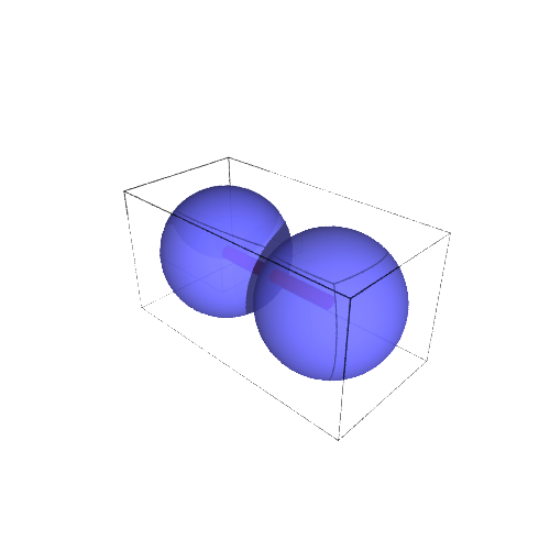
S = sphere(opacity=0.8, aspect_ratio=[1,1,1])
L = line3d([(0,0,0),(2,0,0)], thickness=10, color='red')
M = S + S.translate((2,0,0)) + L
M.show(viewer='tachyon')
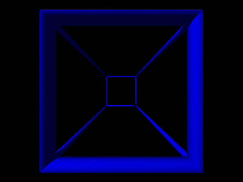
cedges = [[[1, 1, 1], [-1, 1, 1]], [[1, 1, 1], [1, -1, 1]],[[1, 1, 1], [1, 1, -1]], [[-1, 1, 1], [-1, -1, 1]], [[-1, 1, 1],[-1, 1, -1]], [[1, -1, 1], [-1, -1, 1]], [[1, -1, 1], [1, -1, -1]],[[-1, -1, 1], [-1, -1, -1]], [[1, 1, -1], [-1, 1, -1]],[[1, 1, -1], [1, -1, -1]], [[-1, 1, -1], [-1, -1, -1]],[[1, -1, -1], [-1, -1, -1]]]
t = Tachyon(xres=800, yres=600, camera_center=(-1.5,0.0,0.0), zoom=.2)
t.texture('t1', color=(0,0,1))
for ed in cedges:
    t.fcylinder(ed[0], ed[1], .05, 't1')
t.light((-4,-4,4), .1, (1,1,1))
t.show()
%var r,u,v
f=u*v; urange=(u,0,pi); vrange=(v,0,pi)
T = (r*cos(u)*sin(v), r*sin(u)*sin(v), r*cos(v), [u,v])
T = (r*cos(u),r*sin(u),z,[r,u])
rrange=(r,0,2)
plot3d(1, rrange, urange, transformation=T,mesh=1)
3D rendering not yet implemented
plot3d?
File: /ext/sage/sage-8.4_1804/local/lib/python2.7/site-packages/sage/plot/plot3d/plot3d.py
Signature : plot3d(f, urange, vrange, adaptive=False, transformation=None, **kwds)
Docstring :
Plots a function in 3d.

INPUT:

* "f" - a symbolic expression or function of 2 variables

* "urange" - a 2-tuple (u_min, u_max) or a 3-tuple (u, u_min,
  u_max)

* "vrange" - a 2-tuple (v_min, v_max) or a 3-tuple (v, v_min,
  v_max)

* "adaptive" - (default: False) whether to use adaptive
  refinement to draw the plot (slower, but may look better). This
  option does NOT work in conjunction with a transformation (see
  below).

* "mesh" - bool (default: False) whether to display mesh grid
  lines

* "dots" - bool (default: False) whether to display dots at mesh
  grid points

* "plot_points" - (default: "automatic") initial number of sample
  points in each direction; an integer or a pair of integers

* "transformation" - (default: None) a transformation to apply.
  May be a 3 or 4-tuple (x_func, y_func, z_func, independent_vars)
  where the first 3 items indicate a transformation to Cartesian
  coordinates (from your coordinate system) in terms of u, v, and
  the function variable fvar (for which the value of f will be
  substituted). If a 3-tuple is specified, the independent
  variables are chosen from the range variables.  If a 4-tuple is
  specified, the 4th element is a list of independent variables.
  "transformation" may also be a predefined coordinate system
  transformation like Spherical or Cylindrical.

Note: "mesh" and "dots" are not supported when using the Tachyon
  raytracer renderer.

EXAMPLES: We plot a 3d function defined as a Python function:

   sage: plot3d(lambda x, y: x^2 + y^2, (-2,2), (-2,2))
   Graphics3d Object

We plot the same 3d function but using adaptive refinement:

   sage: plot3d(lambda x, y: x^2 + y^2, (-2,2), (-2,2), adaptive=True)
   Graphics3d Object

Adaptive refinement but with more points:

   sage: plot3d(lambda x, y: x^2 + y^2, (-2,2), (-2,2), adaptive=True, initial_depth=5)
   Graphics3d Object

We plot some 3d symbolic functions:

   sage: var('x,y')
   (x, y)
   sage: plot3d(x^2 + y^2, (x,-2,2), (y,-2,2))
   Graphics3d Object

   sage: plot3d(sin(x*y), (x, -pi, pi), (y, -pi, pi))
   Graphics3d Object

We give a plot with extra sample points:

   sage: var('x,y')
   (x, y)
   sage: plot3d(sin(x^2+y^2),(x,-5,5),(y,-5,5), plot_points=200)
   Graphics3d Object

   sage: plot3d(sin(x^2+y^2),(x,-5,5),(y,-5,5), plot_points=[10,100])
   Graphics3d Object

A 3d plot with a mesh:

   sage: var('x,y')
   (x, y)
   sage: plot3d(sin(x-y)*y*cos(x),(x,-3,3),(y,-3,3), mesh=True)
   Graphics3d Object

Two wobby translucent planes:

   sage: x,y = var('x,y')
   sage: P = plot3d(x+y+sin(x*y), (x,-10,10),(y,-10,10), opacity=0.87, color='blue')
   sage: Q = plot3d(x-2*y-cos(x*y),(x,-10,10),(y,-10,10),opacity=0.3,color='red')
   sage: P + Q
   Graphics3d Object

We draw two parametric surfaces and a transparent plane:

   sage: L = plot3d(lambda x,y: 0, (-5,5), (-5,5), color="lightblue", opacity=0.8)
   sage: P = plot3d(lambda x,y: 4 - x^3 - y^2, (-2,2), (-2,2), color='green')
   sage: Q = plot3d(lambda x,y: x^3 + y^2 - 4, (-2,2), (-2,2), color='orange')
   sage: L + P + Q
   Graphics3d Object

We draw the "Sinus" function (water ripple-like surface):

   sage: x, y = var('x y')
   sage: plot3d(sin(pi*(x^2+y^2))/2,(x,-1,1),(y,-1,1))
   Graphics3d Object

Hill and valley (flat surface with a bump and a dent):

   sage: x, y = var('x y')
   sage: plot3d( 4*x*exp(-x^2-y^2), (x,-2,2), (y,-2,2))
   Graphics3d Object

An example of a transformation:

   sage: r, phi, z = var('r phi z')
   sage: trans=(r*cos(phi),r*sin(phi),z)
   sage: plot3d(cos(r),(r,0,17*pi/2),(phi,0,2*pi),transformation=trans,opacity=0.87).show(aspect_ratio=(1,1,2),frame=False)

An example of a transformation with symbolic vector:

   sage: cylindrical(r,theta,z)=[r*cos(theta),r*sin(theta),z]
   sage: plot3d(3,(theta,0,pi/2),(z,0,pi/2),transformation=cylindrical)
   Graphics3d Object

Many more examples of transformations:

   sage: u, v, w = var('u v w')
   sage: rectangular=(u,v,w)
   sage: spherical=(w*cos(u)*sin(v),w*sin(u)*sin(v),w*cos(v))
   sage: cylindric_radial=(w*cos(u),w*sin(u),v)
   sage: cylindric_axial=(v*cos(u),v*sin(u),w)
   sage: parabolic_cylindrical=(w*v,(v^2-w^2)/2,u)

Plot a constant function of each of these to get an idea of what it
does:

   sage: A = plot3d(2,(u,-pi,pi),(v,0,pi),transformation=rectangular,plot_points=[100,100])
   sage: B = plot3d(2,(u,-pi,pi),(v,0,pi),transformation=spherical,plot_points=[100,100])
   sage: C = plot3d(2,(u,-pi,pi),(v,0,pi),transformation=cylindric_radial,plot_points=[100,100])
   sage: D = plot3d(2,(u,-pi,pi),(v,0,pi),transformation=cylindric_axial,plot_points=[100,100])
   sage: E = plot3d(2,(u,-pi,pi),(v,-pi,pi),transformation=parabolic_cylindrical,plot_points=[100,100])
   sage: @interact
   ....: def _(which_plot=[A,B,C,D,E]):
   ....:     show(which_plot)
   <html>...

Now plot a function:

   sage: g=3+sin(4*u)/2+cos(4*v)/2
   sage: F = plot3d(g,(u,-pi,pi),(v,0,pi),transformation=rectangular,plot_points=[100,100])
   sage: G = plot3d(g,(u,-pi,pi),(v,0,pi),transformation=spherical,plot_points=[100,100])
   sage: H = plot3d(g,(u,-pi,pi),(v,0,pi),transformation=cylindric_radial,plot_points=[100,100])
   sage: I = plot3d(g,(u,-pi,pi),(v,0,pi),transformation=cylindric_axial,plot_points=[100,100])
   sage: J = plot3d(g,(u,-pi,pi),(v,0,pi),transformation=parabolic_cylindrical,plot_points=[100,100])
   sage: @interact
   ....: def _(which_plot=[F, G, H, I, J]):
   ....:     show(which_plot)
   <html>...
spherical_plot3d?
File: /ext/sage/sage-8.4_1804/local/lib/python2.7/site-packages/sage/plot/plot3d/plot3d.py
Signature : spherical_plot3d(f, urange, vrange, **kwds)
Docstring :
Plots a function in spherical coordinates.  This function is
equivalent to:

   sage: r,u,v=var('r,u,v')
   sage: f=u*v; urange=(u,0,pi); vrange=(v,0,pi)
   sage: T = (r*cos(u)*sin(v), r*sin(u)*sin(v), r*cos(v), [u,v])
   sage: plot3d(f, urange, vrange, transformation=T)
   Graphics3d Object

or equivalently:

   sage: T = Spherical('radius', ['azimuth', 'inclination'])
   sage: f=lambda u,v: u*v; urange=(u,0,pi); vrange=(v,0,pi)
   sage: plot3d(f, urange, vrange, transformation=T)
   Graphics3d Object

INPUT:

* "f" - a symbolic expression or function of two variables.

* "urange" - a 3-tuple (u, u_min, u_max), the domain of the
  azimuth variable.

* "vrange" - a 3-tuple (v, v_min, v_max), the domain of the
  inclination variable.

EXAMPLES:

A sphere of radius 2:

   sage: x,y=var('x,y')
   sage: spherical_plot3d(2,(x,0,2*pi),(y,0,pi))
   Graphics3d Object

The real and imaginary parts of a spherical harmonic with l=2 and
m=1:

   sage: phi, theta = var('phi, theta')
   sage: Y = spherical_harmonic(2, 1, theta, phi)
   sage: rea = spherical_plot3d(abs(real(Y)), (phi,0,2*pi), (theta,0,pi), color='blue', opacity=0.6)
   sage: ima = spherical_plot3d(abs(imag(Y)), (phi,0,2*pi), (theta,0,pi), color='red', opacity=0.6)
   sage: (rea + ima).show(aspect_ratio=1)  # long time (4s on sage.math, 2011)

A drop of water:

   sage: x,y=var('x,y')
   sage: spherical_plot3d(e^-y,(x,0,2*pi),(y,0,pi),opacity=0.5).show(frame=False)

An object similar to a heart:

   sage: x,y=var('x,y')
   sage: spherical_plot3d((2+cos(2*x))*(y+1),(x,0,2*pi),(y,0,pi),rgbcolor=(1,.1,.1))
   Graphics3d Object

Some random figures:

   sage: x,y=var('x,y')
   sage: spherical_plot3d(1+sin(5*x)/5,(x,0,2*pi),(y,0,pi),rgbcolor=(1,0.5,0),plot_points=(80,80),opacity=0.7)
   Graphics3d Object

   sage: x,y=var('x,y')
   sage: spherical_plot3d(1+2*cos(2*y),(x,0,3*pi/2),(y,0,pi)).show(aspect_ratio=(1,1,1))
spherical_plot3d(2,(x,0,pi/2),(y,0,pi))
3D rendering not yet implemented
cylindrical_plot3d?
File: /ext/sage/sage-8.4_1804/local/lib/python2.7/site-packages/sage/plot/plot3d/plot3d.py
Signature : cylindrical_plot3d(f, urange, vrange, **kwds)
Docstring :
Plots a function in cylindrical coordinates.  This function is
equivalent to:

   sage: r,u,v=var('r,u,v')
   sage: f=u*v; urange=(u,0,pi); vrange=(v,0,pi)
   sage: T = (r*cos(u), r*sin(u), v, [u,v])
   sage: plot3d(f, urange, vrange, transformation=T)
   Graphics3d Object

or equivalently:

   sage: T = Cylindrical('radius', ['azimuth', 'height'])
   sage: f=lambda u,v: u*v; urange=(u,0,pi); vrange=(v,0,pi)
   sage: plot3d(f, urange, vrange, transformation=T)
   Graphics3d Object

INPUT:

* "f" - a symbolic expression or function of two variables,
  representing the radius from the z-axis.

* "urange" - a 3-tuple (u, u_min, u_max), the domain of the
  azimuth variable.

* "vrange" - a 3-tuple (v, v_min, v_max), the domain of the
  elevation (z) variable.

EXAMPLES:

A portion of a cylinder of radius 2:

   sage: theta,z=var('theta,z')
   sage: cylindrical_plot3d(2,(theta,0,3*pi/2),(z,-2,2))
   Graphics3d Object

Some random figures:

   sage: cylindrical_plot3d(cosh(z),(theta,0,2*pi),(z,-2,2))
   Graphics3d Object

   sage: cylindrical_plot3d(e^(-z^2)*(cos(4*theta)+2)+1,(theta,0,2*pi),(z,-2,2),plot_points=[80,80]).show(aspect_ratio=(1,1,1))
%var theta
cylindrical_plot3d(z,(theta,0,2*pi),(z,-2,2),plot_points=[80,80],mesh=1,).show(aspect_ratio=(1,1,1),spin=1)
3D rendering not yet implemented
e=plot(e^x,(x,-5,0) )
f=plot(1+x+x^2/2+x^3/6+x^4/24,(x,-5,0))
show(e+f)
