Thermal Systems HW 3.sagews

import numpy as np
T = 1600 #in Kelvin
#variable will be listed in order in arrays ie. [a,b,c,d]
#values from A.9
Rbar = 8.31451 #universal gas constant
nu = np.array([1,1,2], dtype=float)
h_form = np.array([0,0,90291], dtype=float)
deltah = np.array([41904,44267,43319], dtype=float)
sbar = np.array([244.139,260.434,265.019],dtype=float)
g = (h_form+deltah)-T*(sbar)
DeltaG = (nu[2]*g[2])-(nu[1]*g[1])-(nu[0]*g[0])
K = e**(-DeltaG/(Rbar*T))
print(ln(K))

-10.546697881173996

%typeset_mode True
#in this problem, Sum of nu_i = 0
%var x
ntot = 2
gamm_2(x) = x
gamm_1(x) = (1-x)/2
gamm_0(x) = (1-x)/2
roots = solve([K == gamm_2**nu[2]/(gamm_1**nu[1]*gamm_0**nu[0])],x,solution_dict=True)
roots = [s[x] for s in roots]
num_roots = map(n, roots)
holder = []
for roots in num_roots:
    if roots >= 0:
        holder.append(roots)
x = holder
print ('x=', x)
print('Equilibrium composition is the following:')
pretty_print('yN2, yO2, yNO', (gamm_0(x[0]),gamm_1(x[0]),gamm_2(x[0])))

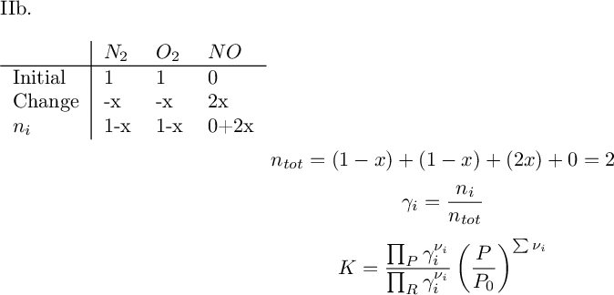
('x=', [0.00255665363707503]) Equilibrium composition is the following:

yN2, yO2, yNO ($\displaystyle 0.498721673181462$, $\displaystyle 0.498721673181462$, $\displaystyle 0.00255665363707503$)

K_conc10 = ln(gamm_2(.1)**nu[2]/((gamm_1(.1)**nu[1])*(gamm_0(.1)**nu[0])))
pretty_print('ln(K) when NO is at 10 percent concentration=', K_conc10)
lin_int_T = (K_conc10-(-3.781))/(-2.217-(-3.781))*(200)+2800
pretty_print('Using Table A.11, find the temperature that corresponds, which is equal to', lin_int_T, 'K')

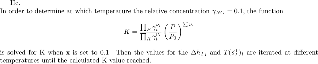
ln(K) when NO is at 10% concentration= $\displaystyle -3.00815479355255$

Using Table A.11, find the temperature that corresponds, which is equal to $\displaystyle 2898.82931028740$ K

P0 = 100
T0 = 298.15
P=500
T=1600

%var x1,x2,x3
#number of moles incorporating dissociation reactions
nH20(x1,x2,x3) = 9
nO2(x1,x2,x3) = (2*12.5)+x1 -x2 -2*x3
nN2(x1,x2,x3) = (141) -x2 -x3
nCO2(x1,x2,x3) = 8-2*x1
nCO(x1,x2,x3) = 2*x1
nNO(x1,x2,x3) = 2*x2
nNO2(x1,x2,x3) = 2*x3
ntot(x1,x2,x3) = nCO2 +nH20 + nN2 + nO2 + nCO + nNO + nNO2


#Equilibrium constant at 1600K from A.11
K1 = e^(-21.656)
K2 = e^(-10.547)
K3 = e^(-20.126)

#mole fractions
yA1 = nCO2/ntot
yC1 = nCO/ntot
yD1 = nO2/ntot

yA2 = nN2/ntot
yB2 = nO2/ntot
yC2 = nNO/ntot

yA3 = nN2/ntot
yB3 = nO2/ntot
yC3 = nNO2/ntot

#nu values
vA1 = 2
vC1 = 2
vD1 = 1

vA2 = 1
vB2 = 1
vC2 = 2

vA3 = 1
vB3 = 2
vC3 = 2

f1(x1,x2,x3)= (yC1^vC1*yD1^vD1) / (yA1^vA1)*(P/P0)^(vC1+vD1-vA1)-K1
f2(x1,x2,x3)= (yC2^vC2) / (yA2^vA2*yB2^vB2)*(P/P0)^(vC2-vB2-vA2)-K2
f3(x1,x2,x3)= (yC3^vC3) / (yA3^vA3*yB3^vB3)*(P/P0)^(vC3-vB3-vA3)-K3
solutions = solve([f1, f2,f3],x1,x2,x3,solution_dict=True,to_poly_solve=True)
pretty_print(solutions)

[$\displaystyle \left\{x_{1} : -1.1014254923 \times 10^{-09}, x_{2} : -0.305450129042, x_{3} : 183.0\right\}$, $\displaystyle \left\{x_{1} : -1.1014254923 \times 10^{-09}, x_{2} : 0.307965711896, x_{3} : 183.0\right\}$, $\displaystyle \left\{x_{1} : 1.1014254923 \times 10^{-09}, x_{2} : -0.305450129042, x_{3} : 183.0\right\}$, $\displaystyle \left\{x_{1} : 1.1014254923 \times 10^{-09}, x_{2} : 0.307965711896, x_{3} : 183.0\right\}$, $\displaystyle \left\{x_{1} : -1.11049643899 \times 10^{-09}, x_{2} : -0.305450129042, x_{3} : 183.0\right\}$, $\displaystyle \left\{x_{1} : -1.11049643899 \times 10^{-09}, x_{2} : 0.307965711896, x_{3} : 183.0\right\}$, $\displaystyle \left\{x_{1} : 1.11049643776 \times 10^{-09}, x_{2} : -0.305450129042, x_{3} : 183.0\right\}$, $\displaystyle \left\{x_{1} : 1.11049643776 \times 10^{-09}, x_{2} : 0.307965711896, x_{3} : 183.0\right\}$, $\displaystyle \left\{x_{1} : -341, x_{2} : 0, x_{3} : -158\right\}$]

pretty_print('f1',f1)
pretty_print('f2',f2)
pretty_print('f3',f3)

f1 $\displaystyle \left( x_{1}, x_{2}, x_{3} \right) \ {\mapsto} \ \frac{5 \, {\left(x_{1} - x_{2} - 2 \, x_{3} + 25.0000000000000\right)} x_{1}^{2}}{{\left(x_{1} - x_{3} + 183.000000000000\right)} {\left(x_{1} - 4\right)}^{2}} - 3.93476409623126 \times 10^{-10}$

f2 $\displaystyle \left( x_{1}, x_{2}, x_{3} \right) \ {\mapsto} \ -\frac{4 \, x_{2}^{2}}{{\left(x_{1} - x_{2} - 2 \, x_{3} + 25.0000000000000\right)} {\left(x_{2} + x_{3} - 141\right)}} - 0.0000262721792989793$

f3 $\displaystyle \left( x_{1}, x_{2}, x_{3} \right) \ {\mapsto} \ -\frac{4 \, {\left(x_{1} - x_{3} + 183.000000000000\right)} x_{3}^{2}}{5 \, {\left(x_{1} - x_{2} - 2 \, x_{3} + 25.0000000000000\right)}^{2} {\left(x_{2} + x_{3} - 141\right)}} - 1.81714363504325 \times 10^{-9}$

# substituting the solutions in the fn equations gives very low values. That's good, I guess …

for sol in solutions:
    print f1.subs(sol)(x1,x2,x3), f2.subs(sol)(x1,x2,x3), f3.subs(sol)(x1,x2,x3)
 37eebf48-8f86-4318-92a8-6a95caf49e46

Error in lines 1-2 Traceback (most recent call last): File "/projects/sage/sage-6.10/local/lib/python2.7/site-packages/smc_sagews/sage_server.py", line 904, in execute exec compile(block+'\n', '', 'single') in namespace, locals File "", line 2, in <module> File "sage/symbolic/expression.pyx", line 4811, in sage.symbolic.expression.Expression.substitute (/projects/sage/sage-6.10/src/build/cythonized/sage/symbolic/expression.cpp:27729) self._gobj.subs_map(smap, 0)) ValueError: power::eval(): division by zero