CoCalc -- MIWsmi1Dv2.sagews

###MIWsim1D###

Author: D Cyganski

Created: 2015-05-17

%auto
%default_mode octave

####Implementation of Wiseman many interacting worlds simulation for 1D, 1 Particle systems####

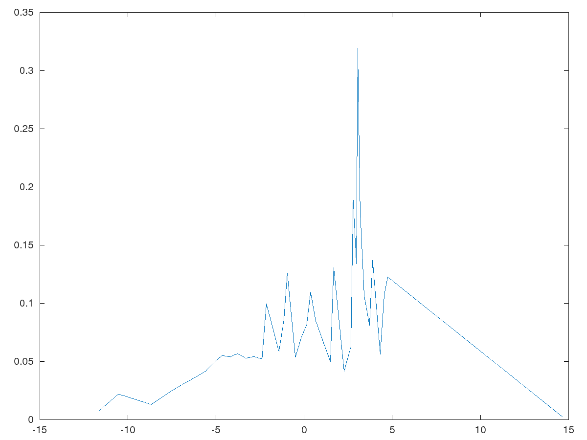
v1 - demo of packet spreading and Fresnel diffraction of 1D packet with spreading
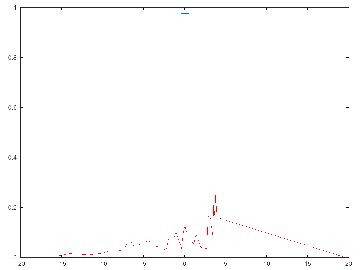
v2 - single particle with gaussian distribution and nonzero mean velocity, colliding with a potential barrier
v3 - single particle in two gaussian superposition with velocities, colliding with no interacting fields

The future track of the many worlds position state $Xp(t)=[x_1(t)...x_{N*J*D}(t)]$ is determined in general in MIW by system of $N*J*D$ coupled non-linear second order partial differential equations, where $N$ =number of worlds, $J$ =number of particles, $D$ =number of dimensions. $m_k*\ddot{x}_{kn}(t) = f_k(x_n(t)) + r_{kN}(x_n(t);Xp(t))$ where $k$ indexes the particle and $n$ the world.

Such a system of $N*J*D$ second order non-linear PDEs can always be written as a system of of $2*N*J*D$ first order linear PDEs:

\dot{x}_{kn}(t) = y_{kn}(t) \\ \dot{y}_{kn}(t) = (1/m_k)*(f_k(x_n(t)) + r_{kN}(x_n(t))

which in turn can be put into matrix state-system form for state vector X=[x, y]'

\dot{X}(t) = Ac*X(t)+Fc(t)+Rc(t)

where I have suppressed the non-linear functional dependencies of $F$ and $R$ , and incorporated the mass scaling into the new function $Fc$ $Rc$ and stacked all the particles and worlds into the single vector

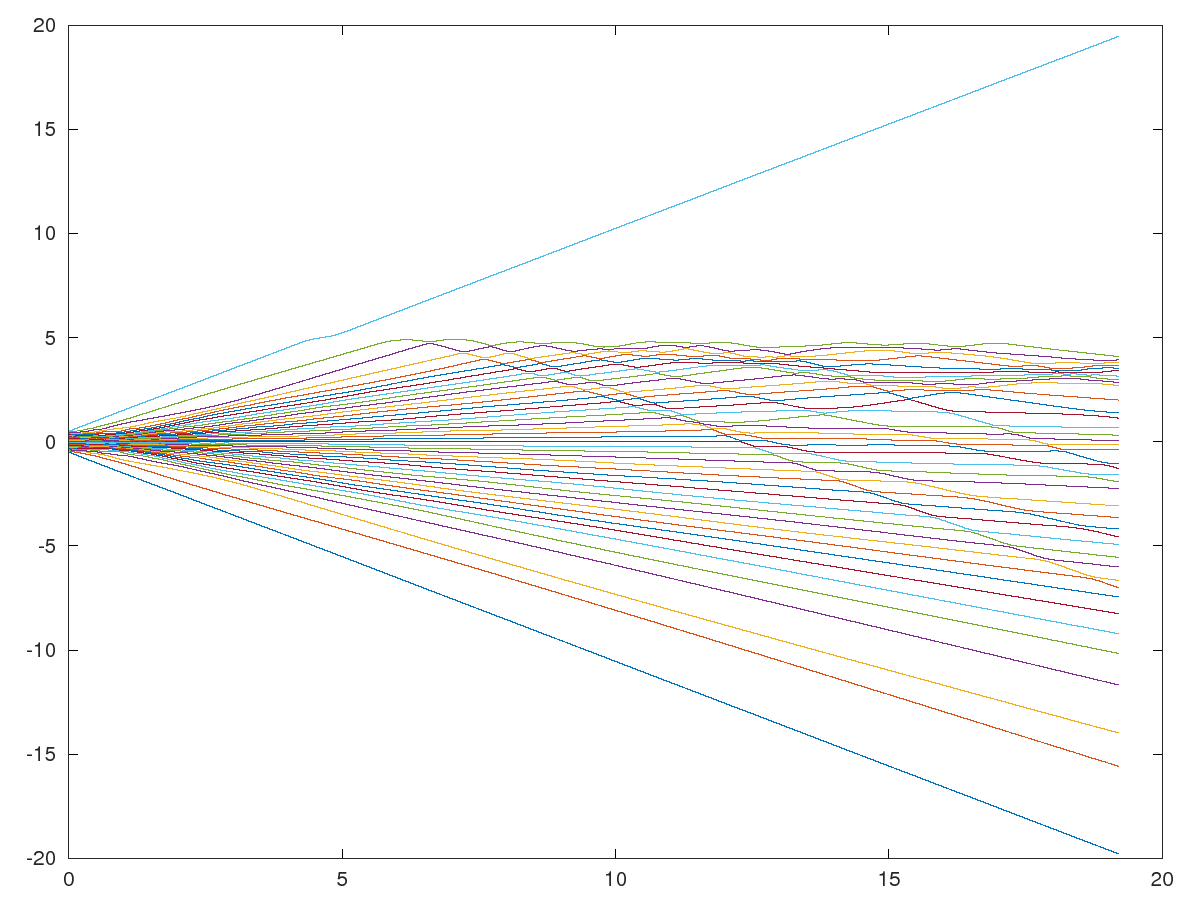
We will now discretize this matrix differential equation and introduce the discrete time state vector of positions and velocities ( $x$ and $\dot{x}$ ) to be named $X$ .

For our 1 D case, there will be $N$ equations. $X$ has $2N$ state variables (position, velocity) In a discrete state space representation, the system is described as $2N$ first order linear state transition equations, and is representable as a $2N$ dimenstional matrix state space equation.

clear all;

%Generate initial distribution of particle states, including position,x, and velocity, xdot
% X=[x1,x2,....xN,x1dot,x2dot,...xNdot]'
% X=InitialGaussian1D(N,0,1,1); %(worlds, center, width, velocity)

%For a simple test, distribute 101 values equally over a window and set all velocities to zero
%xvalues=[-1:.05:1]'; %Prob2
%xvalues=[-1:.025:1]'; %Prob3
xvalues=[-0.5:.025:0.5]'; %Prob4

%xuniform=[-0.95:0.1:0.95]'; %For the simple test

%octave
%xuniform=[-0.95:0.025:0.95]';
%Use inverse error function to generate a Gaussian distribution of trajectories
%xvalues=erfcinv(xuniform);
%xvalues=erfinv(xuniform);
N=size(xvalues,1); %Number of worlds
X = [xvalues; zeros(N,1)]; %zero initial velocities
%X = [xvalues; ones(N,1)]; %non-zero initial velocities

h = figure('visible', 'off');
%Plot the input trajectory density
Pin=(N*(xvalues(2:N,1)-xvalues(1:(N-1),1))).^(-1);
plot(xvalues(2:N,1),Pin);
%xlim([-1,1]); ylim([0,1]);
saveas(h,"figure1.png");

%sage salvus.file("figure1.png")

Now use the appropriate state propagation matrix to step this system forward in time. $X(n+1)=A*X(n)+F(x_n)+R(x_n,X)$ with $A=expm(Ac*T)$ ; where $Ac$ is the continuous time state propagation matrix, $T$ is the time interval between time steps, and expm is octave's matrix exponentiation function.

Note: The HDW paper does not explicitly use the matrix exponentiation based conversion of the continuous time to discrete time conversion. While a naive conversion produces results that converge to the same solution as $T$ approaches 0, for any finite value of $T$ , the exponentiation approach will produce solutions closer to that of the un-discretized system of equations.

I discovered that when I applied the exponentiation to the Ac matrix, thanks to the fact that the differential equations involved did not involve any state variables in its linear part, the outcome of expm(Ac) yields the most simple (naive) summation equation. Since the matrix A that results is extremely sparse, it is computationally advantageous to simply use direct for loop implementation than matrix multiplication.

T=24000; %number of time steps to compute
dT=0.08e-2; %time interval of a single step
m =1; %mass of particle
hbar=.1; %Planck constant %.02 works but nonguassian after 500 iterations

%Reserve recording space
Xrec=zeros(N,T);

%Define a force field at from x=4.9 to 5.1 which repells the oncoming particles
%F=inline("0"); %Simply allow the initial pulse to evolve
%F=inline("ifelse((x>4.7)&&(x<5.3), -0.8, 0)"); %For the simple test
F=inline("ifelse((x>4.7)&&(x<5.3), ifelse(x<5,-1.5,1.5), 0)"); %Triangular potential

t0 = clock ();

%Perform time updates
for t=1:T

%Update the y (==xdot) values
for n=(N+1):(2*N)
  R=MIWforce(N,n-N,X(1:N),m,hbar); %Equations 24,25 of HEW paper
  X(n)=X(n)+(F(X(n-N))+R)*dT;
endfor;
%Update the x values
for n=1:N
  X(n)=X(n)+X(n+N)*dT;
  %Record the position state for plotting
  Xrec(:,t)=X(1:N,1);
endfor;
endfor; t

elapsed_time = etime (clock (), t0)

t =  24000
elapsed_time =  694.00

trec=[1:T]'*dT;
h = figure('visible', 'off');
plot(trec,Xrec);
saveas(h,"figure2.png");
%ylim([-2,2]);

%sage salvus.file("figure2.png")

h = figure('visible', 'off');
%Plot the density at the end of the simulation
Dist=((Xrec(2:N,T)-Xrec(1:(N-1),T)));
Prob=(1/N)*Dist.^(-1);
plot(Xrec(2:N,T),Prob);
saveas(h,"figure3.png");
%xlim([-1.5,1.5]); ylim([0,1]);

%sage salvus.file("figure3.png")

h = figure('visible', 'off');
%Plot the density at 3/4 through the simulation
Tsamp=3*T/4;
Dist=((Xrec(2:N,Tsamp)-Xrec(1:(N-1),Tsamp)));
Prob=(1/N)*Dist.^(-1);

Inline plot failed, consider trying another graphics toolkit
error: print: no axes object in figure to print
error: called from
    _make_figures>safe_print at line 122 column 7
    _make_figures at line 44 column 13

plot(Xrec(2:N,Tsamp),Prob);
saveas(h,"figure4.png");
%xlim([-1.5,1.5]); ylim([0,1]);

%sage salvus.file("figure4.png")

h = figure('visible', 'off');
Dist=((Xrec(2:N,T)-Xrec(1:(N-1),T)));
Prob=(1/N)*Dist.^(-1);
plot(xvalues(2:N,1),Pin);
hold on
Dist=((Xrec(2:N,T)-Xrec(1:(N-1),T)));
Prob=(1/N)*Dist.^(-1);
plot(Xrec(2:N,T),Prob,"r");
saveas(h,"figure5.png");
hold off

%sage salvus.file("figure5.png")

figure("visible","off");
moviename="MIW1D.mp4";
movie("init",moviename)
for Tsamp=1:10:T
Dist=((Xrec(2:N,Tsamp)-Xrec(1:(N-1),Tsamp)));
Prob=Dist.^(-1);
plot(Xrec(2:N,Tsamp),Prob);
xlim([-20,20]); ylim([0,20]);
movie("add",moviename); 
endfor
movie("close",moviename,40); %last arg is frame rate

GPL Ghostscript 9.18: **** Could not open the file 'MIW1D.d/000237.png'.
GPL Ghostscript 9.18: Unrecoverable error, exit code 1
error: save: unable to open output file 'MIW1D.d/+frame-number+'
error: called from
    movie at line 82 column 7
error: load: unable to find file MIW1D.d/+frame-number+
error: called from
    movie at line 102 column 9

%sage salvus.file("MIW1D.mp4")

Error in lines 1-1
Traceback (most recent call last):
  File "/cocalc/lib/python2.7/site-packages/smc_sagews/sage_server.py", line 1009, in execute
    exec compile(block+'\n', '', 'single') in namespace, locals
  File "", line 1, in <module>
  File "/cocalc/lib/python2.7/site-packages/smc_sagews/sage_server.py", line 838, in file
    file_uuid = self._conn.send_file(filename)
  File "/cocalc/lib/python2.7/site-packages/smc_sagews/sage_server.py", line 167, in send_file
    f = open(filename, 'rb')
IOError: [Errno 2] No such file or directory: u'MIW1D.mp4'