exemplo-20.1-seção-20.sagews

%md
## Exemplo 20.1 da Seção 20

Exemplo 20.1 da Seção 20

A = 5
B = 3
C = 5

x, y = var('x y')
phi(x,y) = A*x^2 + 2*B*x*y + C*y^2
phi

(x, y) |--> 5*x^2 + 6*x*y + 5*y^2

c = 1

phi(x,y) == c

5*x^2 + 6*x*y + 5*y^2 == 1

xmin = -1
xmax = 1
ymin = -1
ymax = 1
pcurva = implicit_plot(phi(x,y) - c, (x, xmin, xmax), (y, ymin, ymax))
pcurva.show(axes_labels=['$X$', '$Y$'], axes=True)

M = Matrix([[A, B], [B, C]])
M

[5 3] [3 5]

z = var('z')

solve(z^2 - (A+C)*z + A*C-B^2 == 0, z)

[z == 2, z == 8]

M.eigenvalues()

[8, 2]

lambda1, lambda2 = M.eigenvalues()

lambda1

8

lambda2

2

D, P = M.eigenmatrix_right()

D

[8 0] [0 2]

P

[ 1 1] [ 1 -1]

w1 = vector(P[:,0])
w2 = vector(P[:,1])

w1

(1, 1)

w2

(1, -1)

u1 = (1/w1.norm())*w1
u2 = (1/w2.norm())*w2

u1

(1/2*sqrt(2), 1/2*sqrt(2))

u2

(1/2*sqrt(2), -1/2*sqrt(2))

u1.dot_product(u2)

0

p1 = arrow((0,0), u1, color='green', legend_label='u1', legend_color='black')
p2 = arrow((0,0), u2, color='red', legend_label='u2', legend_color='black')
pS = arrow((-1,1), (1,-1), linestyle='--', width=1, color='black')
pT = arrow((-1,-1), (1,1), linestyle='--', width=1, color='black')
tS = text("S", (1.1, -0.9), color='black')
tT = text("T", (1.1, 0.9), color='black')
p = p1 + p2 + pcurva + pS + pT + tS + tT
p.show(aspect_ratio=1,axes_labels=['$X$', '$Y$'], xmin=xmin, xmax=xmax+0.5, ymin=ymin, ymax=ymax, axes=True, gridlines=True)

a = u2[0]
b = u2[1]

a

1/2*sqrt(2)

b

-1/2*sqrt(2)

theta = var('theta')
solve([cos(theta) == a, sin(theta) == b], theta)

[[theta == -1/4*pi + 2*pi*z42]]

s, t = var('s t')

X = a*s - b*t
Y = b*s + a*t

phibarra(s,t) = phi(X,Y).simplify_full()
phibarra

(s, t) |--> 2*s^2 + 8*t^2

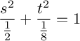
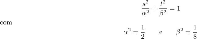
phibarra(s,t) == c

2*s^2 + 8*t^2 == 1

pcurvaST = implicit_plot(phibarra(s,t) - c, (s, xmin, xmax), (t, ymin, ymax))
pcurvaST.show(axes_labels=['$S$', '$T$'], axes=True)

%latex
$$\frac{s^2}{\frac{1}{2}} + \frac{t^2}{\frac{1}{8}} = 1$$

%latex
$$\frac{s^2}{\alpha^2} + \frac{t^2}{\beta^2} = 1$$
com
$$\alpha^2 = \frac{1}{2} \qquad \mathrm{e} \qquad \beta^2 = \frac{1}{8}$$

%latex
No sistema de coordenadas $OST$, sejam $F' = (-\gamma,0)$ e $F = (\gamma,0)$ os focos da elipse.
Então
$$\gamma = \sqrt{\alpha^2 - \beta^2}$$

alpha = sqrt(1/2)
beta = sqrt(1/8)
gamma = sqrt(alpha^2 - beta^2)

gamma

1/2*sqrt(3/2)

Flinha = point((-gamma, 0))
F = point((gamma, 0))
tFlinha = text("F'", (-gamma, -0.1), color='black')
tF = text("F", (gamma, -0.1), color='black')

p = pcurvaST + Flinha + F + tFlinha + tF
p.show(axes_labels=['$S$', '$T$'], axes=True)

X(s,t) = a*s - b*t
Y(s,t) = b*s + a*t

X

(s, t) |--> 1/2*sqrt(2)*s + 1/2*sqrt(2)*t

Y

(s, t) |--> -1/2*sqrt(2)*s + 1/2*sqrt(2)*t

FlinhaXY = X(-gamma,0), Y(-gamma,0)
FXY = X(gamma,0), Y(gamma,0)

FlinhaXY

(-1/4*sqrt(2)*sqrt(3/2), 1/4*sqrt(2)*sqrt(3/2))

FXY

(1/4*sqrt(2)*sqrt(3/2), -1/4*sqrt(2)*sqrt(3/2))

pFlinhaXY = point(FlinhaXY)
pFXY = point(FXY)
tFlinhaXY = text("F'", (FlinhaXY[0], FlinhaXY[1] - 0.1), color='black')
tFXY = text("F", (FXY[0] - 0.1, FXY[1]), color='black')

p = pcurva + pFlinhaXY + pFXY + pS + pT + tS + tT + tFlinhaXY + tFXY
p.show(aspect_ratio=1, axes_labels=['$X$', '$Y$'], xmin=xmin, xmax=xmax+0.2, ymin=ymin, ymax=ymax, axes=True, gridlines=True)